INTERNATIONAL MONETARY FUND. Navigating Global Divergences (October 2023)

WORLD ECONOMIC OUTLOOK: Navigating Global Divergences

Box 1.1. Dimming Growth Prospects: A Longer Path to Convergence

Since the global financial crisis in 2008, forecasters

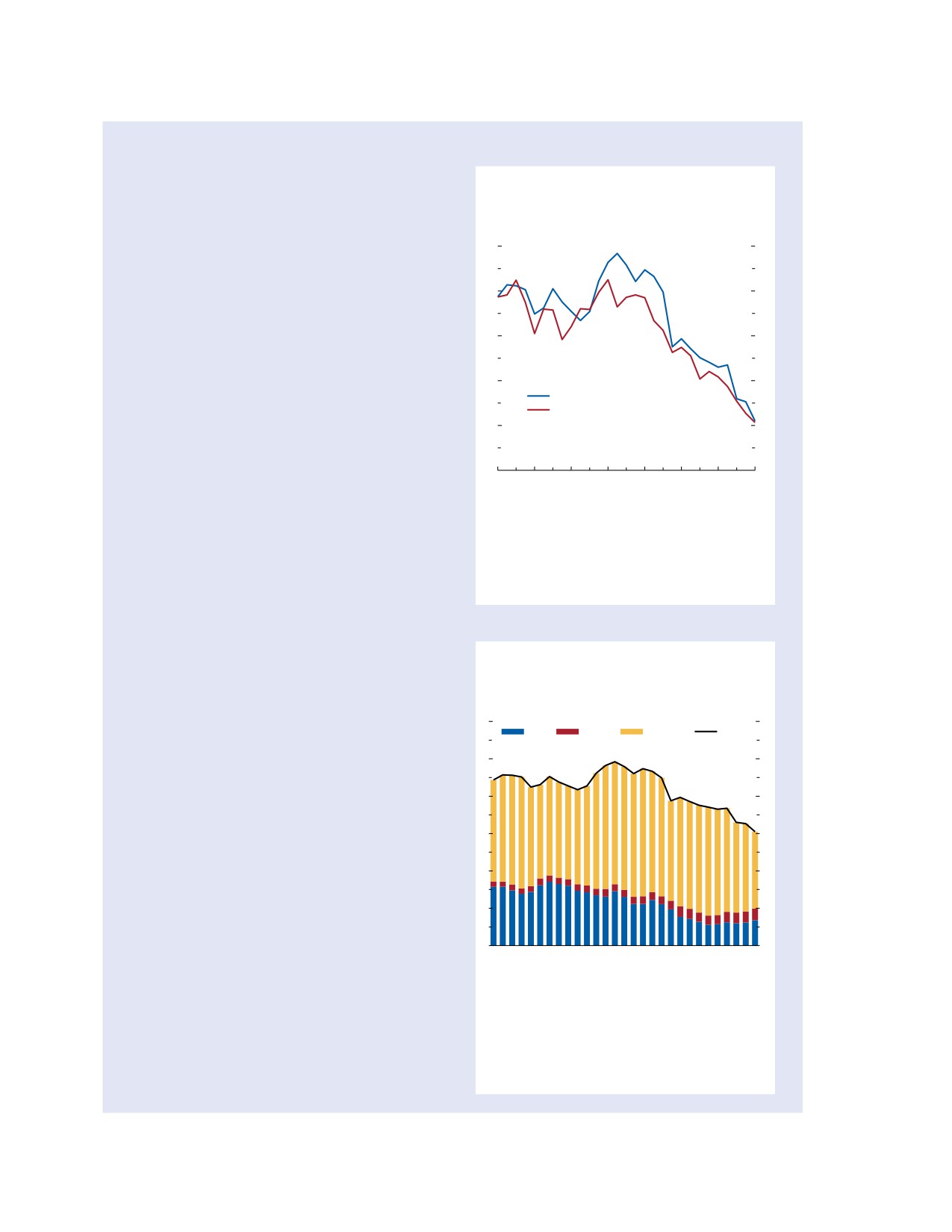
Figure 1.1.1. Five-Year-Ahead Growth

have steadily diminished their expectations for growth

Projections

over the medium term. Global five-year-ahead growth

(Percent)

projections from the World Economic Outlook (WEO)

have declined from a peak of 4.9 percent in the April

5.0

2008 WEO for growth in 2013 to 3.0 percent in the

April 2023 WEO for growth in 2028: the lowest pro-

4.5

jection since 1990 (Figure 1.1.1). Forecasters at other

institutions—as surveyed by Consensus Economics--

4.0

have similarly reduced their expectations. If the focus

is WEO forecasts, the decline in growth prospects

started in the early 2000s for advanced economies,

3.5

while emerging market and developing economies

World Economic Outlook

Consensus Economics

experienced a similar decline after the crisis. Of the

3.0

1.9 percentage point global decline in medium-term

growth prospects from 2008 to 2023, advanced

economies contributed 0.8 percentage point; emerg-

2.5

2000

ing market and developing economies contributed

1.1 percentage points. Among emerging market and

Sources: Consensus Economics; and IMF staff calculations.

developing economies, low-income developing coun-

Note: The predicted variable is real GDP growth. The years

on the horizontal axis refer to the year for which a forecast is

tries increased their contribution to projected global

made, using the April World Economic Outlook (WEO) five

growth slightly during the same period (Figure 1.1.2).

years prior, such that, for example, the 2028 forecast is

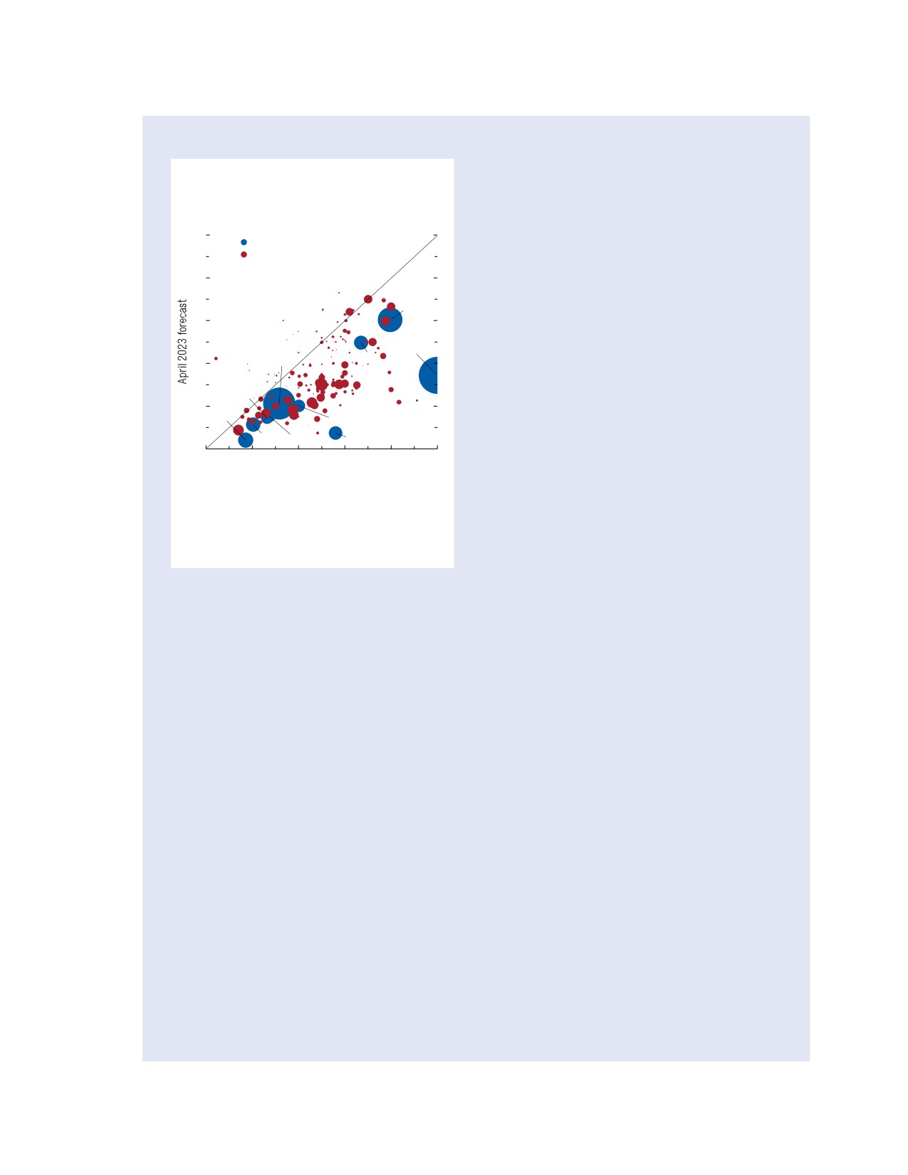
Te world’s largest 10 economies, and 81 percent of all

based on the April 2023 WEO, and so on. The red line

depicts the mean of the Consensus Economics forecasts.

economies, have seen a decline in their medium-term

growth prospects (Figure 1.1.3). Te five largest

emerging markets--Brazil, China, India, Indonesia,

and Russia--have contributed about 0.9 percentage

Figure 1.1.2. Five-Year-Ahead Growth

point to the decline in medium-term global growth

Projections: Country Groups

(Percent)

prospects between 2008 and 2023. East Asia and the

Pacific’s outlook has seen the largest downshift. Te

global medium-term outlook further declined after

AEs

LIDCs

EMMIEs

World

the shocks of 2020-22—including the COVID-19

pandemic and the Russian invasion of Ukraine--from

3.6 percent in the January 2020 WEO to 3.0 percent

in the April 2023 WEO, with 52 percent of econo-

mies (all of them middle-income economies) seeing

a decline.

A natural question is whether the decline in

forecasters’ expectations for the global economy over

the past 15 years has been excessively pessimistic,

with outcomes likely to be better than expected. An

examination of the bias in WEO forecast errors over

time--the average difference between actual outcomes

2000

and forecasts--suggests that the answer is no. Forecasts

Source: IMF staff calculations.

were mostly aligned with growth outcomes during

Note: The predicted variable is real GDP growth. The years

1995-2008. After the global financial crisis, forecasts

on the horizontal axis refer to the year for which a forecast is

exhibited--if anything--some upward bias, with

made, using the April World Economic Outlook (WEO) five

years prior, such that, for example, the 2028 forecast is

realized growth over the medium term falling short

based on the April 2023 WEO, and so on. AEs = advanced

economies; EMMIEs = emerging market and middle-income

economies; LIDCs = low-income developing countries.

Te authors of this box are Nan Li and Diaa Noureldin.

International Monetary Fund | October 2023

CHAPTER 1 Global Prospects and Policies

Box 1.1 (continued)

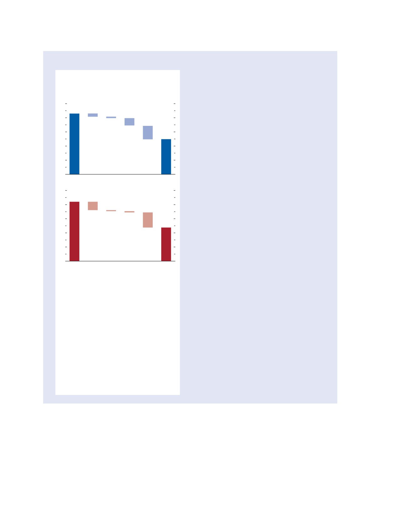
For advanced economies, the decline in per capita

Figure 1.1.3. Projected Growth Deceleration

output growth in the recent forecasts relative to the

in the Largest Economies

forecasts for the early 2000s is attributed predomi-

(Five-year-ahead GDP growth, percent)

nantly to lower TFP growth, followed by the decline

in labor force participation and the slowdown in

Top 10 economies in 2028

Other economies

capital deepening (Figure 1.1.4). Tis reflects fore-

casters’ views on future TFP growth, potentially due

to unbalanced technological advances across sectors

IND

(Acemoglu, Autor, and Patterson 2023), frictions

preventing efficient resource allocation (Baqaee and

Farhi 2020), or diminishing returns to innovation

CHN

USA

IDN

(Bloom and others 2020). Te projected decline in

the contribution of labor force participation, which is

FRA

broad-based across advanced economies, could reflect

JPN

forecasters’ views on the impact of population aging.

BRA

GBR

Te decline in the contribution of capital deep-

DEU

RUS

ening could reflect views on declining investment

prospects over time, partly on account of scarring

April 2008 forecast

effects on capital formation after the global financial

Source: IMF staff calculations.

crisis, and is most pronounced in regard to euro

Note: The predicted variable is real GDP growth. Bubble size

area economies.³ For emerging market and devel-

indicates GDP in purchasing-power-parity international

oping economies, the decline in TFP growth is also

dollars for 2028. Data labels in the figure use International

Organization for Standardization (ISO) country codes.

the largest contributor to the slowdown, explaining

about 60 percent, followed by the decline in capital

deepening. Te projected decline in TFP growth in

of medium-term predictions.¹ Tis suggests that the

emerging market and developing economies could

downward trajectory in the projections could in part

reflect fading effects of technological and educational

reflect correcting for forecast optimism since the crisis.

improvement, the slowdown in reform momentum

A deeper look through forecasters’ lenses sheds

in the 2000s relative to the 1990s (October 2019

light on the factors driving the decline. First,

WEO), and rising fragmentation risks that would

three-quarters of the reduction in global growth

hurt growth in world trade and global value chains.

prospects (about 1.4 percentage points) over the past

Te projected slowdown in capital deepening is

15 years has come from weaker per capita growth

also a significant contributor in some of the largest

projections rather than merely slower population

emerging market and developing economies—

growth. Second, it is instructive to note that per

such as Brazil and Indonesia.⁴

capita growth can be decomposed into changes in

Te decline in medium-term growth prospects,

capital per worker (or “capital deepening”), labor

especially in emerging market and developing econ-

force participation, the employment rate (employ-

omies, has worrisome implications for the pace of

ment as a share of the labor force), and total factor

convergence in living standards. Fifteen years ago,

productivity (TFP) (see Abiad and others 2009).²

¹Te assessment is based on the regression e 

= α + ε 

³Te scarring effects of the global financial crisis on invest-

i,t

i,t, in

which e 

ment are documented in the April 2015 World Economic

i,t is the growth forecast error, defined as the five-year

end-of-period moving average of realized growth rates minus

Outlook. A potential explanation is the relatively larger fiscal

the five-year-ahead forecast, conducted as a vintage-by-vintage

consolidation in euro area economies after the crisis. Tis may

regression over the period 1990-2017, with the last vintage

have prompted expectations of a slower rate of capital accumula-

chosen to compare against the output realization for 2022. Te

tion, given evidence suggesting strong complementarity between

results are robust to using actual growth rates instead of the

public and private investment in European economies (Brasili

moving average.

and others 2023).

²Te term capturing labor force participation also reflects

⁴Tese trends are generally consistent with estimates of

changes in the share of the working age population in

potential output growth (see, for instance, Kilic Celik, Kose, and

total population.

Ohnsorge 2023).

International Monetary Fund | October 2023

WORLD ECONOMIC OUTLOOK: Navigating Global Divergences

Box 1.1 (continued)

the five-year-ahead growth forecasts in the April 2008

Figure 1.1.4. Per Capita Growth Forecast

WEO implied a positive and statistically significant

Decomposition

rate of absolute convergence--with poorer countries

(Percent)

growing unconditionally faster than rich countries

2.5

1. Advanced Economies

by 0.9 percent annually. At this rate of convergence,

economies’ progress in raising their living standards

2.0

and the associated decline in the rate of change

Capital

EMP.

deepening

might have been expected to translate into a decline

rate

LFP

1.5

in global growth over time. Accordingly, IMF staff

TFP

estimates suggest that up to 0.4 percentage point of

1.0

the aforementioned decline in per capita global growth

0.5

prospects since 2008 may reflect income convergence.⁵

In contrast, the five-year-ahead growth forecasts in

0.0

the April 2023 WEO imply a convergence rate of

2000-04

2024-28

only 0.5 percent a year, corresponding to the flatter

5.0

2. Emerging Market and Developing Economies

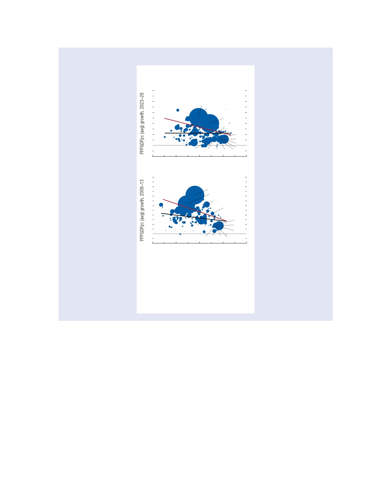
relationship shown in Figure 1.1.5. Tese forecasts

imply that the expected number of years needed for

4.0

emerging market and developing economies to close

half the gap in income per capita with advanced econ-

Capital

EMP.

LFP

3.0

deepening rate

omies has significantly increased. For example, based

on the population-weighted estimates in Figure 1.1.5,

2.0

TFP

this half-life estimate has on average increased from

80 years for projections in the April 2008 WEO to

1.0

about 130 years for projections in the April 2023

0.0

WEO. What is more, these estimates are population

2000-04

2024-28

weighted, meaning that they give greater weight to

more populous and faster-growing countries, such as

Sources: Penn World Table version 10.01; and IMF staff

calculations.

China and India. Unweighted regressions—indicated

Note: The dark red and blue bars represent the period

in the figure by black lines—show even slower

average of projected five-year-ahead per capita growth

expected convergence rates that decline to near zero

rates. The light red and blue bars represent the

contributions, in percentage-point changes, to the total

in the April 2023 WEO projections. Poorer countries

reduction in per capita growth between 2000-04 and

have already suffered greater income losses during the

2024-28. The sample includes countries for which a full set

recovery from the pandemic (Brussevich, Liu, and

of projections is available for all included variables and

represents about 60 percent of world GDP at purchasing

Papageorgiou 2022). Te slower prospects for income

power parity in 2023. The World Economic Outlook (WEO)

convergence suggest a particularly difficult road ahead.

database includes forecasts for gross fixed capital

formation, which were used to construct the capital stock,

with historical depreciation rates taken from the Penn World

⁵Te expected (absolute) convergence rate implied by projec-

Table (assumed constant from 2019 onward). The initial

tions in the April 2008 WEO is 0.3 percent when each country

capital stock is estimated based on the respective

is treated as a unit of analysis and 0.9 percent when countries are

capital-to-output ratios from the Penn World Table and

weighted by population. Applying the 0.3-0.9 range of conver-

assuming a capital share in output equal to 0.35.

gence rates to the level of initial GDP per capita across countries

EMP. = employment; LFP = labor force participation;

in 2008 implies a decline in global per capita GDP growth of

TFP = total factor productivity.

0.1-0.4 percentage point over 2008-23.

International Monetary Fund | October 2023

WORLD ECONOMIC OUTLOOK: Navigating Global Divergences

Box 1.2. Risk Assessment Surrounding the World Economic Outlook’s Baseline Projections

Te IMF’s Group of Twenty (G20) Model is used in

remain relevant for the current outlook, they are

this box to derive confidence bands around the World

evaluated through a scenario instead of a shift in the

Economic Outlook (WEO) forecast and to quantify

predictive distribution. Second, the distribution for

alternative scenarios. Uncertainty about 2023 has

2023 shocks has shrunk as the outturn for the first

narrowed considerably since the April 2023 WEO as

half of the year is already known.

the outturn for the first half of the year is now known.

Figure 1.2.1 (panels 1, 2, and 3) shows the distri-

Beyond 2023, risks to growth are considered more

butions for global growth and inflation projections

balanced than in the April 2023 WEO but still tilted to

that result from the approach and assumptions just

the downside. Te risk of global growth falling below

discussed. Each shade of blue represents a 5 percentage

2 percent—an outcome that has occurred on only five

point interval, and the entire band covers 90 percent

occasions since 1970—in 2024 is assessed at about

of the distribution. Regarding global growth, the range

15 percent, compared with 25 percent in April. Te

of possible outcomes has narrowed and shifted up

balance of risks for inflation beyond 2023 has shifted

relative to April. Tere is a 70 percent probability that

up, reflecting upward revisions to the baseline projec-

global growth will be between 2.6 percent and 3.4 per-

tion. Te risk that core inflation in 2024 will be higher

cent in 2023—a narrower range than in April—and

than in 2023 is assessed at about 15 percent. Te

a 70 percent probability that growth will be between

scenarios assess several risks to the outlook. Upside risks

1.9 percent and 4.0 percent in 2024.

include (1) greater-than-expected disinflation effects

Regarding global inflation, uncertainty around 2023

from fading supply disruptions and (2) a greater boost

has narrowed for both the headline and core figures:

to global demand from a stronger recovery in invest-

there is now a 70 percent probability that 2023

ment in advanced economies. Downside risks include

headline inflation could be about 0.7 percentage point

(1) further loss of growth momentum in China, (2)

higher or lower than currently projected, lower than

longer-than-expected transmission lags and larger effects

the 1.2 percent band shown in April. Beyond 2023,

from the ongoing global monetary tightening cycle, and

risks have tilted up with the revision to the baseline:

(3) tighter financial conditions in emerging markets.

the probability that headline inflation in 2024 will be

higher than in 2023 is assessed at 25 percent, com-

Confidence Bands

pared with less than 10 percent in April. Similarly, the

Te methodology for producing confidence bands

probability that core inflation in 2024 will be higher

is based on Andrle and Hunt (2020) and was used in

than in 2023 is assessed at 15 percent, compared with

the October 2022 and April 2023 WEO reports. Te

about 5 percent back in April.

G20 model, presented in Andrle and others (2015), is

Risk Scenarios

used to interpret historical data on output, inflation,

and international commodity prices and to recover

Te April 2023 WEO presented a single large down-

the implied economic shocks to aggregate demand

side scenario for the world economy, centered around

and supply. Te recovered shocks are sampled through

a large shock to credit supply. While financial risks

non-parametric methods and fed back through the

remain, the probability of a severe scenario from bank-

model to generate predictive distributions around the

ing sector developments has receded. Instead, this box

WEO projections. Distributions for global macro vari-

quantifies several upside and downside risks. While

ables are then obtained by aggregating country-level

each of the risks quantified here implies relatively

estimates. Tere are two changes to the distributions

moderate effects on global growth and inflation, several

for growth and inflation outcomes relative to April.

could materialize at the same time, in which case the

First, shocks from 1982 were sampled more heavily

global impact would be correspondingly larger. Te

in the previous WEO to stress the risk of a more

scenarios assume that monetary policy and automatic

pronounced slowdown from contractionary monetary

fiscal stabilizers respond endogenously to macro devel-

policy. Here instead, shocks are sampled uniformly,

opments, without additional policy support.

consistent with risks to the outlook having become

Upside Risks

more balanced. While risks from monetary policy

Greater-than-expected global disinflation from

Te authors of this box are Jared Bebee, Harri Kemp, Pedro

further supply normalization: Supply constraints

Rodriguez, and Rafael Portillo.

have been an important factor in the global inflation

International Monetary Fund | October 2023

CHAPTER 1 Global Prospects and Policies

Box 1.2 (continued)

surge experienced during the pandemic recovery,

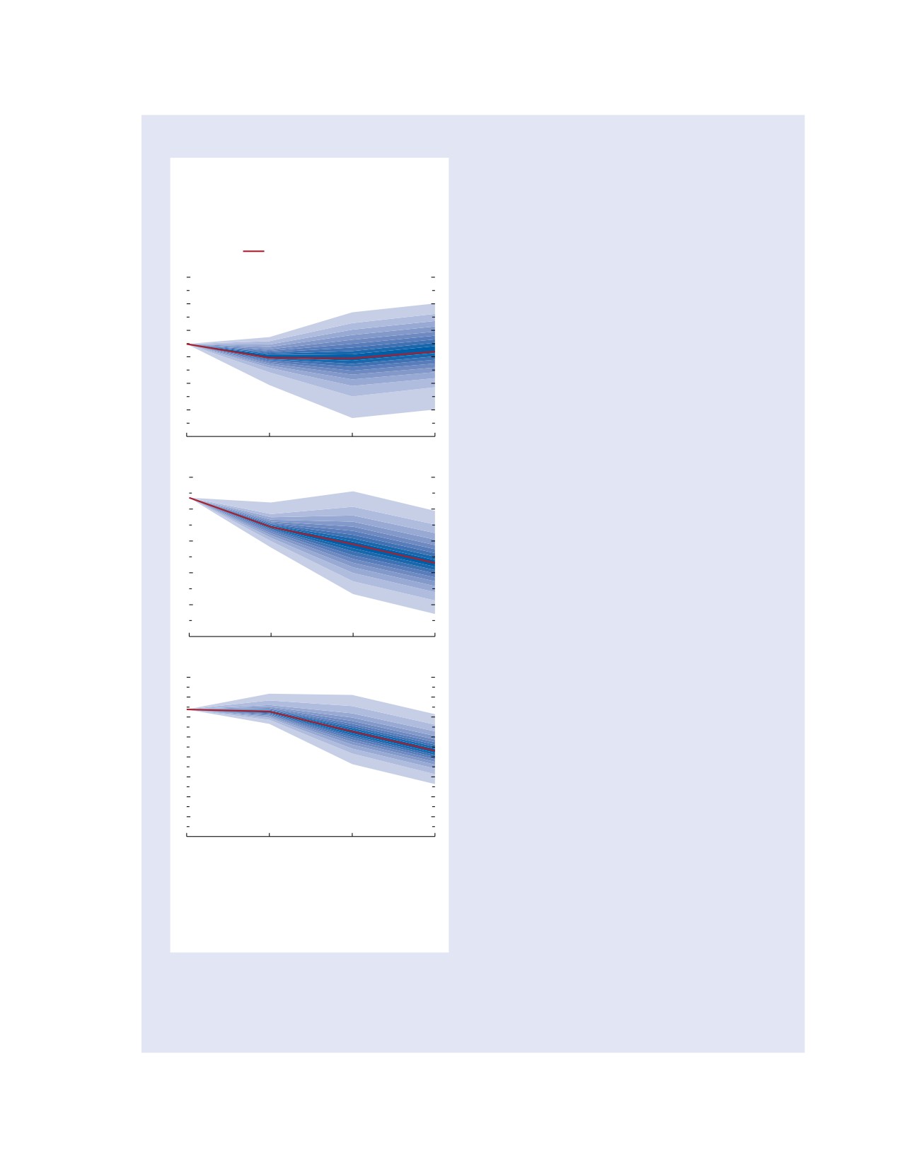
Figure 1.2.1. Distribution of Forecast

both directly through higher goods inflation early on

Uncertainty around Global GDP Growth and

and indirectly by raising marginal costs. As multiple

Inflation Projections

indicators point to normalization, fading supply dis-

(Percent)

ruptions are now helping with the ongoing disinfla-

WEO baseline projection

tion. Te scenario assumes that the global disinflation

impulse is greater than in the baseline forecast, with

1. Real GDP Growth

the consumer price of manufactured goods relative to

services—currently estimated to be 1 percent above

the global aggregate trend prior to the COVID-19

pandemic—returning to trend over a two-year hori-

zon. Te additional impulse in the scenario is larger in

countries, mainly advanced economies, that are start-

ing from a higher relative goods price, with an impulse

equal to -20 basis points of core inflation in 2023 and

-50 basis points in 2024 (relative to baseline). For

2022

the remaining countries, except China, the impulse is

two-thirds as large; China experiences a smaller shock.

2. Headline CPI Inflation

Te lower-than-expected inflation raises purchasing

power globally and allows central banks to lower

rates at a more rapid pace over the scenario horizon,

supporting global consumption, investment, and trade.

Stronger recovery in investment in advanced

economies: Investment has been lagging since the

COVID-19 crisis period ended, with global gross fixed

capital formation remaining close to 10 percent below

prepandemic trends. Te scenario assumes investment

grows by more than in the baseline over the next two

2022

years for several advanced economies, reflecting both

3. Core CPI Inflation

(1) greater sensitivity to the expected recovery in some

regions and sectors, and easing financial conditions,

and (2) a stronger-than-expected boost from current

policy packages (US Inflation Reduction Act, EU

recovery fund). Higher investment supports global

demand and trade but also adds to inflationary pres-

sures, with the added assumption that Phillips curves

are twice as sensitive to demand, as a result of the cur-

rent inflation environment, which elicits a stronger pol-

icy response. However, the increase is modest in size:

2022

in the scenario, investment is 3 percent higher than the

baseline by 2025 for the advanced economies group.

Source: IMF staff calculations.

Note: The figure shows the distribution of forecast

uncertainty around the baseline projection as a fan. Each

Downside Risks

shade of blue represents a 5 percentage point probability

Subdued confidence weighing on China’s out-

interval. CPI = consumer price index; WEO = World

Economic Outlook.

look: Te scenario assumes a deeper-than-expected

contraction in the real estate sector in the absence of

swift action to restructure property developers, weaker

consumption in the context of subdued confidence,

and lack of meaningful policy support. As a result,

China’s private consumption and gross fixed capital

International Monetary Fund | October 2023

WORLD ECONOMIC OUTLOOK: Navigating Global Divergences

Box 1.2 (continued)

formation decline through 2025 by about -5 percent

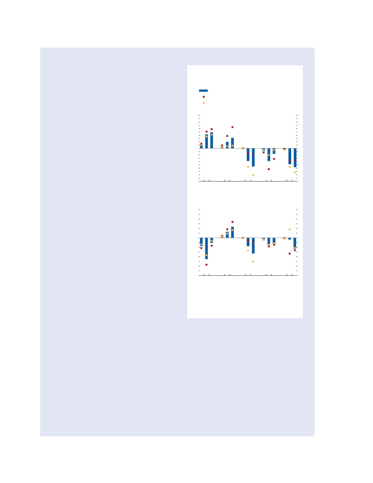
Figure 1.2.2. Impact of Scenario on GDP

and -3.5 percent, relative to baseline. Te shock fades

Level and Core Inflation

beyond 2025.

Longer transmission lags and greater-than-expected

World

effects from global monetary policy tightening: Te

Advanced economies

relative resilience of the global economy in the first

Emerging market and developing economies

half of 2023 has raised the question of whether the

1. Impact on GDP Level

1.0

full effect from the ongoing global monetary tight-

0.8

(Percent deviation from baseline)

ening is yet to be seen. Te scenario assumes that the

0.6

effects are larger than what is in the current WEO

0.4

baseline, that the additional impulse in each coun-

0.2

try is proportional to the change in real rates since

0.0

the beginning of the tightening cycle, and that the

-0.2

effects materialize by the end of 2023—and especially

-0.4

-0.6

in 2024. Te calibration draws on the uncertainty

-0.8

regarding transmission lags and magnitudes from dif-

-1.0

ferent models and empirical estimates. Specifically, the

20232425

232425

shock is calibrated for the United States and the euro

Disinflation

China Monetary Financial

investment

policy

conditions

area by comparing the effects so far from the tight-

ening, from the IMF’s G20 Model—which happen

0.6

2. Impact on Core Inflation

early in the tightening cycle and are smaller—with

(Percentage point deviation from baseline)

0.4

the effects from the FRB/US model and the structural

vector autoregression (SVAR) model in Gertler and

0.2

Karadi (2015) for the United States and ECB-Base

0.0

model for the euro area, which take longer and are

-0.2

generally larger. Te differences between the two

sets of estimates are then fed into the G20 Model as

-0.4

shocks to aggregate demand, resulting in lower activity

-0.6

and inflation and a decrease in the policy rate relative

-0.8

to the baseline. For other G20 countries, the shock to

20232425

232425

Disinflation

China

Monetary Financial

aggregate demand is calculated as the average of the

investment

policy

conditions

US and EU estimates (for each 1 percentage point

increase in the real rate) multiplied by that country’s

Source: IMF staff calculations.

real rate increase. Te estimated shocks to demand

Note: X-axis labels denote five distinct scenarios.

AE = advanced economy.

are largest in advanced economies (Australia, Can-

ada, UK, US) and some emerging market economies

(Brazil, Mexico).

Tighter financial conditions in emerging mar-

into the second half of 2024 and into 2025. Relatedly,

ket economies: While the underlying cause is not

currencies of emerging market economies see a

included in the scenario, tighter financial conditions

depreciation of 10 percent relative to the US dollar in

in emerging markets could result from a combination

the first half of 2024, relative to the baseline.

of higher-for-longer rates in advanced economies,

Impact on World Output and Inflation

especially the United States, and concerns about the

implications for emerging market economies of lower

Figure 1.2.2 (panels 1 and 2) presents the effects

growth in China. Following an incipient tightening

from all four scenarios. Panel 1 shows the effects

toward the end of 2023, emerging market economies,

on GDP for the years 2023, 2024, and 2025, while

excluding China, experience an increase in sovereign

panel 2 shows the effects for inflation over the same

and corporate premiums of about 200 and 150 basis

horizon. Effects on global GDP are presented as

points, respectively, in the first half of 2024, relative

percent deviations from the baseline, while effects on

to the baseline, with some of the tightening persisting

global core inflation are presented as percentage point

International Monetary Fund | October 2023

CHAPTER 1 Global Prospects and Policies

Box 1.2 (continued)

deviations from the baseline.¹ Global aggregates are

••

The downside scenario for China lowers its GDP

shown in bars, while aggregates for advanced econo-

by as much as -1.6 percent in 2025, with a decrease

mies and emerging markets are shown in red squares

in core inflation of about 1 percentage point,

and yellow diamonds, respectively.

relative to the baseline. There are spillovers to

Te scenarios highlight the broadly balanced nature

other countries, and the effect on global output is

of risks to the outlook:

-0.6 percent by 2025.

••

The disinflationary scenario generates a decrease in

••

The scenario of longer monetary lags results in a

global core inflation that troughs at -0.4 percentage

decrease in global output of about -0.4 percent by

point in 2024 relative to the baseline, generating a

2024 and a modest decrease in global core inflation

0.5 percent increase in global GDP in 2024, which

in that year (-0.1 percentage point). The effects

persists into 2025. The effect is somewhat more

are larger in advanced economies: -0.6 percent for

pronounced in advanced economies; as a result,

output and -0.2 percentage point for core inflation.

the latter group sees a decrease in policy rates of

The main reason for the modest impact on inflation

0.3 percentage point, relative to the baseline.

is that policy rates are lowered by 50 basis points in

••

The scenario of stronger recovery in investment in

advanced economies in 2024 relative to the base-

advanced economies generates a modest increase

line, which helps soften the impact.

in global output of up to 0.3 percent by 2025 and

••

Tighter financial conditions in emerging markets

is associated with moderately higher inflation. The

lower the level of global output by -0.5 percent by

impact on GDP in advanced economies peaks at

2024. The effects are more pronounced in emerging

0.6 percent in 2025, adding an additional 0.3 percent-

market economies, but advanced economies are also

age point to core inflation and requiring an increase in

negatively affected because of the loss of compet-

policy rates of about 0.75 percentage point, relative to

itiveness. The inflation responses diverge across

the baseline. Spillovers to emerging markets are small.

country groups initially—the disinflation is initially

muted in emerging market economies, whose

currencies depreciate, and is more pronounced in

¹Te impact on growth rates for a given year can be approxi-

mated by subtracting the effects on the level of output from the

advanced economies, whose currencies appreciate—

previous year.

before converging in 2025.

International Monetary Fund | October 2023

WORLD ECONOMIC OUTLOOK: Navigating Global Divergences

Commodity Special Feature: Market Developments and the

Commodity Price Channel of Monetary Policy

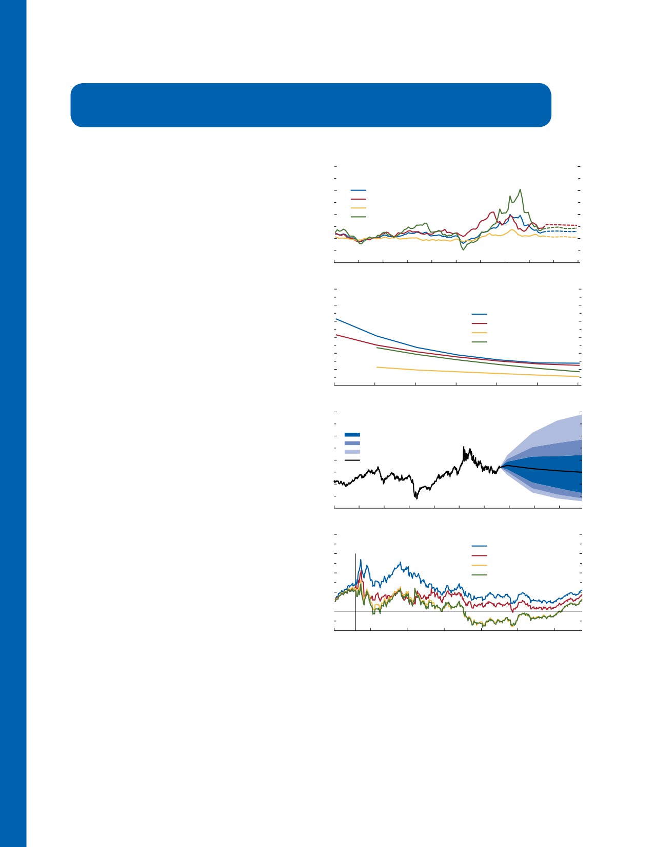
Primary commodity prices declined by 7.5 percent between

Figure 1.SF.1. Commodity Market Developments

February and August 2023. The widespread decline was

400

1. Commodity Price Indices

led by base metals, with prices falling 15.7 percent, and

(CPI adjusted¹)

European natural gas prices, plummeting 36.0 percent.

300

All index

The trend decline in cereal prices was temporarily halted

Base metal index

Food index

by the collapse of the Black Sea Grain Initiative in

200

Energy index

July. Gold prices increased. This Special Feature ana-

lyzes the commodity price channel of monetary policy.

100

2015

Commodity Market Developments

120

2. Brent Prices WEO Forecasts

Supply curbs supporting oil prices. Tanks to

(US dollars a barrel; expiration dates on x-axis)

110

a rebound in July and August, crude oil prices

April 2022 WEO

increased, by 4.4 percent, between February and

100

October 2022 WEO

April 2023 WEO

August 2023, remaining, however, well below their

October 2023 WEO

peak of $115 in June 2022 (Figure 1.SF.1, panels 1

and 3). On the demand side, a weaker-than-expected

rebound in China’s oil consumption, temporary reces-

sion fears because of banking woes, and tighter mon-

2023

etary policy in many major economies all contributed

200

3. Brent Price Medium-Term Prospects³

to downward price pressures, especially in the second

(US dollars a barrel, four-year futures)

quarter of 2023.

150

68 percent confidence interval

86 percent confidence interval

On the supply side, output curbs by OPEC+ (Orga-

95 percent confidence interval

100

Futures

nization of the Petroleum Exporting Countries plus

selected nonmember countries) of 1.2 million barrels

a day (mb/d) announced in April—coupled with

additional voluntary cuts of 1 mb/d and 0.3 mb/d

2017

by Saudi Arabia and Russia, respectively—were only

partly offset by strong oil output growth in non-OPEC

180

4. Brent and Russian Oil Prices⁴

countries, most notably in the United States, where

(US dollars a barrel)

Brent

150

Feb. 24

Russian ESPO (Pacific)

oil output is expected to increase by 1.1 mb/d this

Russian Urals (Black Sea)

year. Western sanctions on Russian crude oil exports

120

Russian Urals (Baltic)

have had mixed effects: export flows of Russian oil

have remained fairly steady, and its price discount

relative to Brent oil has shrunk over time—Russian

$60

oil is trading above the $60 price cap imposed by the

Jan.

Apr.

July

Oct.

Jan.

Apr.

July

Group of Seven (G7) countries—as the size of the

2022

non-Western-aligned oil tanker fleet carrying Russian

oil has increased, and as Russia appears to have set up

Sources: Argus; Bloomberg, L.P.; Haver Analytics; Refinitiv Datastream; IMF,

Primary Commodity Price System; and IMF staff estimates.

its own maritime insurance.

¹US consumer price index adjusted. Last actual value is applied to the forecast.

²Forecasts based on World Economic Outlook (WEO).

³Derived from prices of futures options on August 18, 2023.

⁴Last data point is September 8, 2023. All prices are daily midpoints.

ESPO = Eastern Siberia Pacific Ocean.

Te contributors of this Special Feature are Christian Bogmans,

Wenchuan Dong, Jorge Miranda-Pinto, Andrea Pescatori (Team

Lead), Ervin Prifti, Martin Stuermer, and Guillermo Verduzco-

Bustos with research assistance from Joseph Moussa and Tianchu Qi.

Tis Special Feature is based on Miranda-Pinto and others (2023).

International Monetary Fund | October 2023

Commodity Special Feature MARKET DEVELOPMENTS AND THE COMMODITY PRICE CHANNEL OF MONETARY POLICY

Futures markets suggest that crude oil prices will

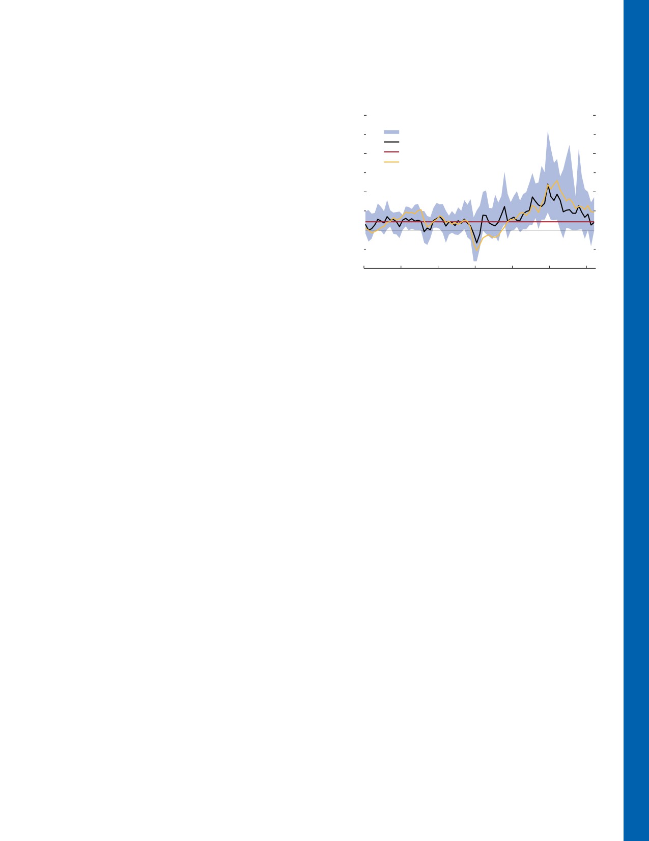
Figure 1.SF.2. Headline Inflation

slide by 16.5 percent year over year to average $80.5 a

(Month-over-month percent change, seasonally adjusted)

barrel in 2023 (from $96.4 in 2022) and continue to

200

fall in coming years, to $72.7 in 2026 (Figure 1.SF.1,

10th to 90th percentile

panel 2). Te International Energy Agency expects oil

Median country

demand to increase by 2.2 mb/d, reaching 102.2 mb/d

Average, 2010-19

150

Oil price (US dollars a barrel, right scale)

in 2023, outstripping supply in the second half of the

year. Uncertainty around this price outlook is elevated

(Figure 1.SF.1, panel 3). Upside price risks stem from

100

additional OPEC+ production cuts, a military escala-

tion in the Black Sea, and insufficient investment in

fossil fuel extraction. Downside price risks stem from

a widespread global economic relapse, a slowdown in

Chinese oil demand, and faster penetration of electric

-10

vehicles.

2017

Natural gas prices continue to normalize. European

Sources: Haver Analytics; IMF, Primary Commodity Price System; and IMF staff

Title Transfer Facility trading hub prices declined

calculations.

36 percent from February to August 2023 to a

Note: Distribution (shaded area) covers countries accounting for 83.9 percent of

World Economic Outlook World GDP (purchasing-power-parity-weighted).

monthly average of $10.7 a million British ther-

mal units (MMBtu) and within the upper range of

historical prices. Lower demand, high storage over-

Reserve’s tightening pace and continued demand for

hang from this past winter, and ample supplies of

inflation hedges and alternatives to the dollar.

liquefied natural gas (LNG) and of pipeline gas from

Agricultural prices continue their downward trend.

Norway and northern Africa have all lowered prices.

Between February and August, the IMF’s food and

Asian LNG prices declined by 26.4 percent, roughly

beverage price index lost 6.7 percent, continuing its

in lockstep with EU prices. US Henry Hub prices

decline, though at a slower pace than in the second

increased by 8.6 percent from February to average

half of 2022. Prices of all major food commodities

$2.6/MMBtu in August 2023. Te price differential

except sugar, rice, and pork contributed to the down-

between US and European gas is expected to slow

ward trend. As a result of a robust supply response in

gradually as US LNG export capacity expansion picks

the 2022-23 season, grain prices fell consistently and

up in 2024 and beyond. Tis is reflected in a slowly

in August stood 20.7 percent lower than in February.

narrowing gap between the US and EU futures price

Grain prices remain, however, 7.7 percent above the

curves. Title Transfer Facility futures prices suggest that

average of the past five years. Food security concerns

average annual prices could move from $13.6/MMBtu

prompted recent export restrictions in India, the

to $17.5/MMBtu in 2024 but then down to $9.1/

world’s largest rice exporter. Risks to prices are tilted

MMBtu by 2028. US Henry Hub prices are expected

to the upside, stemming mostly from the ramifica-

to rise from an annual average of $2.7/MMBtu in

tions of the end of the Black Sea Grain Initiative and

2023 to $3.9/MMBtu in 2028.

uncertain effects of El Niño (see chapter text), pos-

Metal prices have weakened. After a short-lived

sibly exacerbated by the proliferation of food export

rebound during the winter, base metal prices declined by

restrictions.

15.7 percent from February to August as China’s reopen-

ing lost steam and its real estate sector, which together

The Commodity Price Channel of

with construction accounts for roughly 20 percent of

Monetary Policy

global metal consumption, kept faltering (Figure 1.SF.1,

panel 1). Higher interest rates and weak European

Sharp fluctuations in commodity prices, among

industrial demand also contributed to the negative

other factors, have been blamed for the recent global

market sentiment. Forecasts for base metal prices have

surge in inflation and for its subsequent fall (Figure 1.

also been revised downward since the April 2023 World

SF.2) (see, for example, Gagliardone and Gertler 2023;

Economic Outlook, with prices now projected to decline

Blanchard and Bernanke 2023; and Ball, Leigh, and

by 4.7 percent in 2023 and 7.1 percent in 2024. Gold

Mishra 2022). Commodity prices, however, are not

prices remain high following a slowdown in the Federal

exogenous with respect to the macroeconomy. Indeed,

International Monetary Fund | October 2023

WORLD ECONOMIC OUTLOOK: Navigating Global Divergences

part of the recent monetary policy reaction to inflation

storage; (2) a real-economy channel, by affect-

may have operated through a commodity price channel,

ing current and future commodity consumption;

as policy actions from major central banks affect global

(3) a liquidity-and-portfolio channel, by affecting

activity and financial conditions, which are typically

financial conditions and thus trading liquidity in

major drivers of fluctuations in commodity prices.

physical and derivative markets; and (4) an exchange

How quantitatively important is the commodity price

rate channel, as most commodities are traded in

channel of monetary policy—especially US monetary

dollars. Since monetary policy typically has long lags

policy—in driving inflation in the United States and

affecting the real economy, an immediate effect of

worldwide?

a monetary policy shock through the real-economy

Empirical analysis of this question has been limited.¹

channel can work only through expectations and

Tis Special Feature contributes to filling the gap by

thus only for easy-to-store commodities.⁴

estimating the effects of US monetary policy shocks

on commodity prices and, through this channel, their

The Effects of Monetary Policy Shocks on

spillback to the US economy and spillovers to con-

Commodity Prices: A High-Frequency Approach

sumer prices in other countries. It also looks at pass-

through from commodity prices to consumer prices

Local projections are used in the analysis pre-

and potential asymmetries.

sented here to estimate the effects of monetary policy

shocks—as in Jarociński and Karadi (2020)—on

commodity prices.⁵ Te strongest impact is found for

A Conceptual Framework

industrial metals (for example, nickel and copper) and

Among central banks, the Federal Reserve plays a

oil. A 10 basis point monetary policy surprise leads to

special role. Tis is because the bulk of cross-border

a 2.5 percent drop in the base metal price index and

capital flows are denominated in dollars, and US mon-

a 2 percent drop in oil prices, with the peak responses

etary policy is a key driver of the global financial cycle

after about 20 days (see Figure 1.SF.3). Prices for raw

(Dées and Galesi 2021; Miranda-Agrippino and Rey

materials, such as cotton and rubber, also have a sim-

2020). Changes in US interest rates thus have pro-

ilar decline, whereas the reaction of food prices, such

nounced repercussions for the rest of the world (Rey

as those for cereals, is smaller (less than 1 percent) and

2013).² Terefore, this analysis will focus on the effects

less precisely estimated.

of US monetary policy shocks (for an analysis of the

Results are consistent with the cost-of-carry and

effect of European Central Bank shocks, see Online

real-economy channels, as higher interest rates increase

Annex 1.1).³

the opportunity costs of holding inventories and,

Conceptually, US monetary policy can affect

through the delayed effect on economic activity of

commodity prices through (1) a cost-of-carry chan-

higher funding costs, reduce future demand. Tese

nel, by affecting the opportunity cost of commodity

effects are more relevant for commodities with high

storability (for example, base metals).⁶ Te gold price

reaction is very precisely estimated, with the price

¹Recent examples are Breitenlechner, Georgiadis, and Schumann

dropping by 1.1 percent after 23 days. For a given

(2022) and Ider and others (2023).

²Te dollar is both an intervention currency and an anchor cur-

exchange rate, this sets a cap for the cost-of-carry chan-

rency (Gourinchas 2019). Tis helps propagate US monetary policy

nel, since gold prices are moved, during normal times,

impulses from the center to the periphery and provides a common

component to the global monetary environment. Te spillovers of

US monetary policy to the rest of the world are further strengthened

⁴Sizable monetary policy shocks can also have a nonlinear effect

by the importance of dollar funding for global bank balance sheets,

on commodity prices (Miao, Wu, and Funke 2011).

as well as the increasing length and complexity of global supply

⁵Only dollar-denominated commodity prices are considered for

chains (Bruno and Shin 2015).

1990-2019. Te pure monetary policy surprise from Jarociński and

³Policy rate comovement among central banks is elevated. More-

Karadi (2020), which does not consider central bank information

over, US monetary policy shocks seem to lead to policy reactions

effects, is used. More details are presented in Online Annex 1.1.

and policy surprises from other central banks, such as the Bank of

⁶Te responses of natural gas prices (Henry Hub) are not consid-

Canada and the European Central Bank (see Online Annex 1.1 for

ered, as gas markets present important structural changes throughout

details). Kearns, Schrimpf, and Xia (2023) document that spillovers

the sample. For the period 1990-2019, natural gas prices do not

from other central banks are modest. In the case of China, typically

respond to US monetary policy. However, for the 2016-19 subsa-

it is fiscal policy that is more prevalently used for business cycle fluc-

mple only, when US natural gas exports increased dramatically, a

tuations rather than monetary policy. All online annexes are available

significant decline in gas prices after US monetary policy tightening

at www.imf.org/en/Publications/WEO.

is observed.

International Monetary Fund | October 2023

Commodity Special Feature MARKET DEVELOPMENTS AND THE COMMODITY PRICE CHANNEL OF MONETARY POLICY

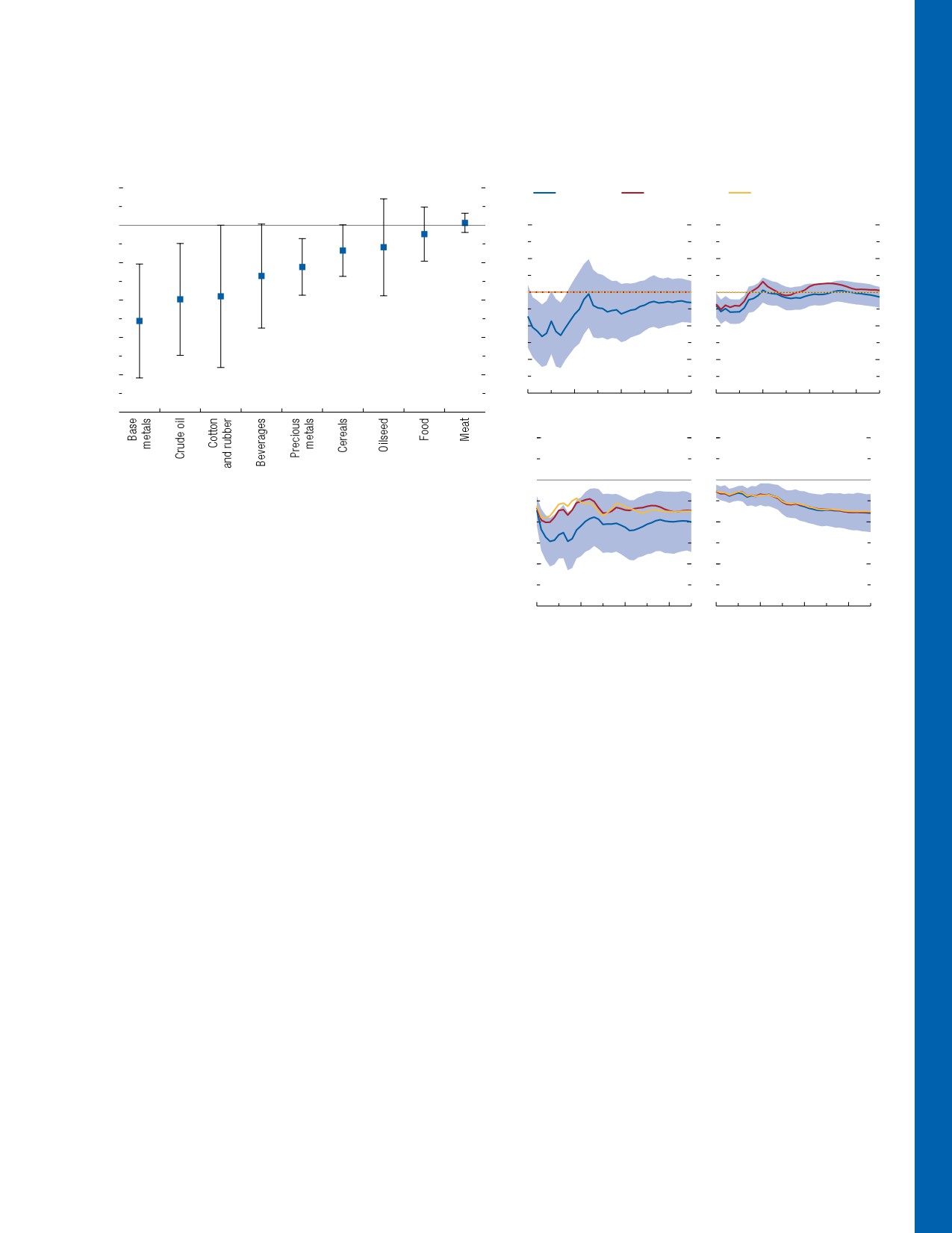
Figure 1.SF.3. Peak Commodity Price Responses to a

Figure 1.SF.4. Impulse Response Functions for a

10-Basis-Point US Monetary Policy Shock

(Percent change)

(Percent)

Benchmark

No oil response

No oil and food responses

1. Oil Price

2. Food Price

-1

–2

-2

–3

-4

-6

–5

0.1

3. Headline CPI

4. Core CPI

0.1

0.0

Sources: Bloomberg L.P.; IMF, Primary Commodity Price System; UN Comtrade;

and IMF staff calculations.

Note: The numbers next to the boxes represent the horizon (day) of the maximum

-0.1

decline in commodity prices. 90 percent error bars are displayed.

-0.2

mostly by the opportunity cost of storing gold.⁷ Mone-

tary policy shocks also affect the dollar, which appreci-

–0.3

-0.3

ates by 0.4 percent, but the impact is short-lived.⁸

Sources: Bloomberg L.P.; Board of Governors of the Federal Reserve System; UN

Comtrade; US Bureau of Labor Statistics; US Energy Information Administration;

The Effects of Monetary Policy Shocks on

and IMF staff calculations.

Note: Red (yellow) lines show the response of the variables under the assumption

Commodity Prices, Spillbacks, and Spillovers

that oil prices (oil and food prices) do not react. Blue areas are 68 percent

confidence bands. Oil and food prices are expressed in current-year dollars.

Next, to gauge domestic spillbacks and spill-

CPI = consumer price index.

overs from US monetary policy to other countries,

a monthly proxy-structural vector autoregression

approach is used. Te analysis first looks at the effects

The Spillbacks

of the commodity price channel on US inflation. It

A 10 basis point increase in the US federal funds

then moves on to the effects on other countries’ infla-

rate induces a decline in oil prices of 2 percent on

tion. Te focus is on prices of food and oil, which have

impact, and the effect persists for eight months. Food

the most direct effects on headline inflation.

prices decline by 1 percent, and the effect is less per-

sistent. Te responses of the headline consumer price

⁷Except in the case of natural gas, the results are robust to choos-

ing different subsample periods, suggesting that the relationship

index (CPI), industrial production, and the exchange

between monetary policy and commodity prices has not changed

rate are in line with the textbook implications of a

over time. Tis remains the case even if the sample is broken into

monetary policy tightening (see Figure 1.SF.4 and

segments before and after 2004, a year typically used to distinguish

between periods before and after the financialization of commodity

Online Annex 1.1).⁹

markets (Tang and Xiong 2012).

⁸Tis suggests that, conditional on a monetary policy shock, the

⁹In addition to the monetary policy instrument, the first specifica-

correlation between the dollar and commodity prices is negative at

tion considers seven macroeconomic variables: the one-year Treasury

high frequencies. Although there is evidence that the unconditional

bill, US headline CPI, US core CPI, US industrial production, the

correlation between commodity prices and the dollar has changed

excess bond premium, the US dollar, the West Texas Intermediate oil

since 2015 (Hofmann, Igan, and Rees 2023), the analysis presented

price, and a food price index. Te data span 1990-2019. Te focus

in this Special Feature does not find evidence of a change in the rela-

on food and energy commodities is because their pass-through to

tionship between US monetary policy and commodity price indices

headline inflation is more direct and less delayed than those of other

for that period (see Online Annex 1.1 for details).

commodities, such as metals, fertilizers, and raw materials.

International Monetary Fund | October 2023

WORLD ECONOMIC OUTLOOK: Navigating Global Divergences

Table 1.SF.1. Average Response of CPIs

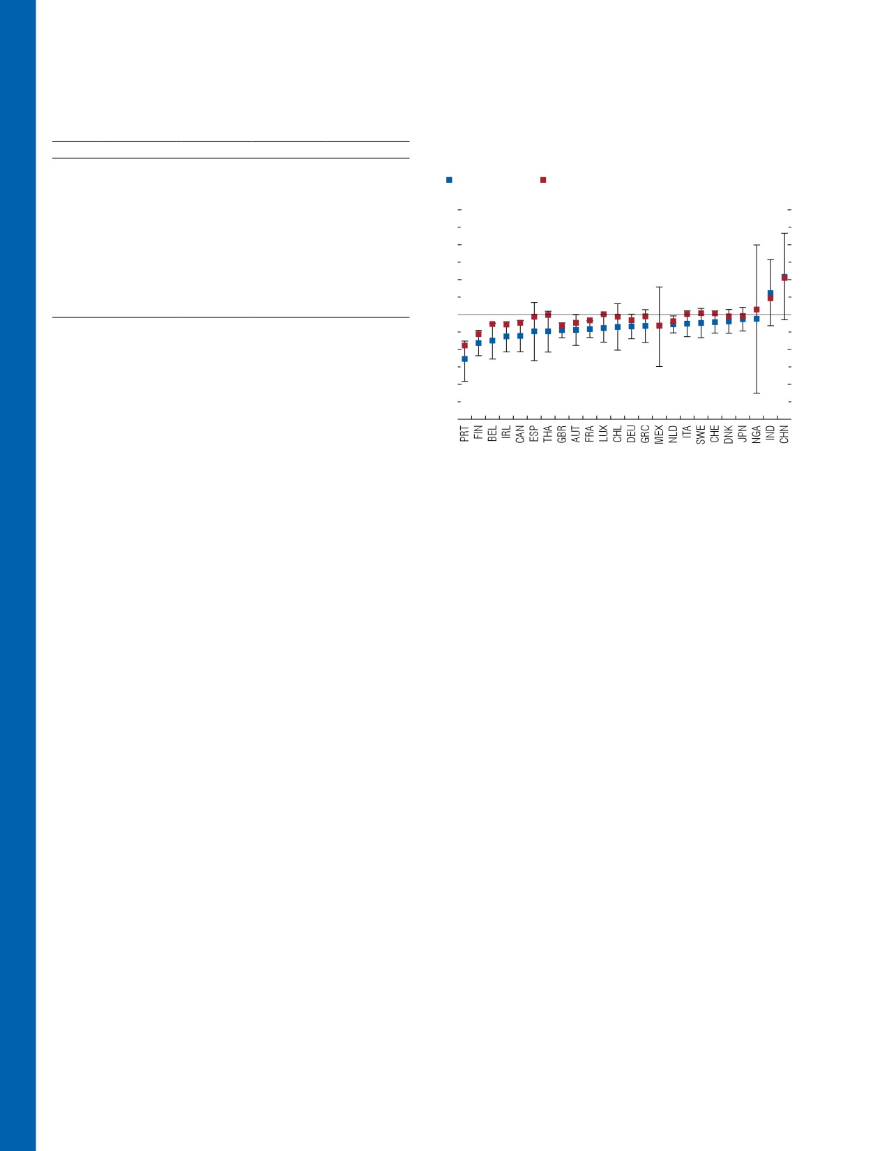
Figure 1.SF.5. Contribution of Oil and Food Prices in the

(Percent)

Transmission of US Monetary Policy Shocks

(Percent)

0-6 Months

0-12 Months

12-24 Months

United

Benchmark

-0.12

-0.02

States

No oil

-0.09

-0.07

-0.02

Response of CPI

Response of CPI when oil and food prices do not react

Contribution¹

(32)

(40)

No oil, no food

-0.07

-0.06

-0.01

0.6

Contribution

(41)

(47)

Contribution MA²

(43)

(40)

0.4

Other

Benchmark

-0.07

Countries No oil

-0.04

-0.03

-0.01

Contribution

(48)

(57)

0.2

No oil, no food

-0.02

Contribution

(66)

(74)

0.0

Sources: Board of Governors of the Federal Reserve System; US Energy Information

Administration; World Bank; and IMF staff calculations.

-0.2

Note: Average response of CPIs to 10 basis point increase in interest rate. Time ranges

in each column are average period of decline. CPI = consumer price index;

MA = Mediation Analysis.

-0.4

¹Percentages in parentheses are contributions of commodity channel.

²“Contribution MA” presents the contribution of the overall commodity index from

-0.6

instrumental variables local projection (IV-LP) mediation analysis (MA).

To isolate the commodity price channel of US

Sources: Board of Governors of the Federal Reserve System; US Energy

monetary policy, in the spirit of Bernanke, Gertler, and

Information Administration; World Bank; and IMF staff calculations.

Watson (1997), the impulse response functions are esti-

Note: Blue and red squares are the average one-year response of CPIs after an

increase of 10 basis points in the US interest rate. Error bars are 68 percent

mated again, with the condition imposed that US mon-

confidence intervals. Data labels in the figure use International Organization for

etary policy has no effect on (1) oil prices and (2) both

Standardization (ISO) country codes. CPI = consumer price index.

oil and food prices. If the commodity price channel is

shut down, US monetary policy has smaller effects on

the CPI. As Table 1.SF.1 shows, absent oil and food

most countries’ CPIs decline after a US monetary

price responses, headline CPI would have declined by

policy tightening. Te role of the commodity price

0.07 percentage point rather than by 0.12 percent-

channel is quantitatively important for several coun-

age point in the first half-year, implying a 41 percent

tries. As highlighted in Table 1.SF.1, for the average

contribution of the commodity price channel. Te

country, the commodity price channel accounts for

contribution is similar for the first year, but it declines

66 percent of the total spillover of US monetary policy

over time as core inflation becomes the main driver (see

onto inflation in the first half-year. Te oil price alone

Figure 1.SF.4, panel 4). Oil prices have a dominant role,

contributes 48 percent.

since oil prices affect food prices but not vice versa.

An instrumental variable-local projection mediation

analysis tends to confirm these results, with an average

Asymmetric Pass-Through

commodity price contribution of 43 percent over a half-

Some observers have suggested that in the most

year period (see Table 1.SF.1 and Online Annex 1.1).

recent episode of heightened inflation, the pass-

through from global commodity prices to domestic

The Spillovers

consumer prices increased. It has also been suggested

Figure 1.SF.5 reports the effects of US monetary

that producers are eager to pass cost changes on to

policy on countries’ CPI (in blue), along with the

consumers when commodity prices are on the rise but

effect of US monetary policy on countries’ CPI absent

refrain from doing so when commodity prices decline.

the commodity price channel (red).¹⁰ As expected,

Finally, producers may also pass a larger fraction of

commodity price changes on to consumer prices when

¹⁰To study the effects of US monetary policy on foreign inflation

through commodity prices, the previous specification is augmented

the changes to commodity prices are larger and happen

with the CPI of country i and the bilateral exchange rate for country

more quickly, attracting the attention of producers by

i and the United States, with the estimate repeated for a set of 24

virtue of their salience.

countries. Te same decomposition is performed to study how much

A series of local projections of domestic food and

of the change in country i’s CPI is due to US monetary policy’s

effect on commodity prices.

energy inflation on food commodity price and oil price

International Monetary Fund | October 2023

Commodity Special Feature MARKET DEVELOPMENTS AND THE COMMODITY PRICE CHANNEL OF MONETARY POLICY

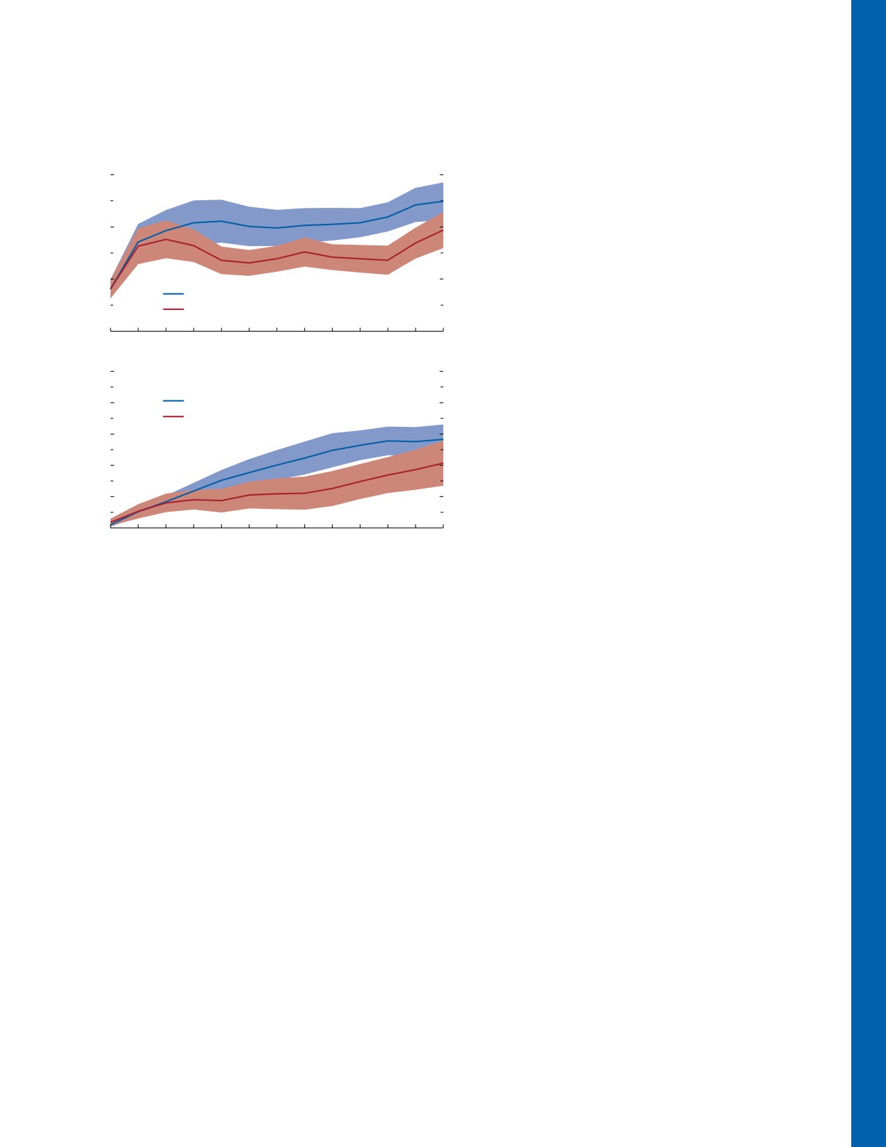
Figure 1.SF.6. Asymmetric Pass-Through of Commodity Price

inflation, there is also evidence that the food price

Shocks

pass-through is heightened for larger and thus more

(Percent)

salient shocks (Figure 1.SF.6, panel 2).

0.3

1. Response of Energy Inflation to 1 Percent Increase in Global

Oil Prices

Conclusions

0.2

Monetary policy has a strong direct effect on

commodity prices, especially those of industrial and

storable commodities such as oil and metals. Spillbacks

0.1

and spillovers to other countries from US monetary

Estimate for large global oil price movements

policy shocks are fast. After a 10 basis point monetary

Estimate for small global oil price movements

policy shock, the decline in oil and food prices over

0.0

the course of six months reduces both domestic and

other countries’ inflation by 0.05 percent on average.

0.5

2. Response of Energy Inflation to 1 Percent Increase in Global

Tis result implies that the commodity price channel

Food Prices

of US monetary policy has relatively larger spillovers

0.4

Estimate for large global food price movements

to other countries than spillbacks to the United States.

Estimate for small global food price movements

0.3

Whereas the commodity price channel accounts for

41 percent of the total decline in US headline CPI, it

0.2

accounts for 66 percent of the total decline in headline

CPI for the average country in the sample.

0.1

Spillovers from US monetary policy shocks tend to

0.0

be more relevant for consumer prices in other advanced

economies, whereas the reaction of consumer prices in

emerging market economies and their commodity price

Sources: Ha, Kose, and Ohnsorge (2021); and IMF staff calculations.

Note: Shaded area is 90 percent confidence interval. Numbers on x-axis represent

channels are less precisely estimated, as emerging markets

months after shock. Coefficient on large (small) price movements estimated on

tend to have more regulated prices. Tere is no signifi-

subsample of price changes larger than (smaller or equal to) one standard

deviation.

cant commodity price channel for core inflation. Major

central banks, when setting policy objectives, should

consider their spillbacks and spillovers through a com-

shocks are conducted to test these hypotheses. For food

modity price channel and expect stronger pass-through

inflation, there is no evidence that the pass-through

during times of sharp commodity price changes (relative

is higher during commodity price booms than busts

to times of small changes). Finally, as the Federal Reserve

or that the pass-through for price increases is larger

tends to set the tone for the global monetary policy

than that for price decreases. However, some evidence

stance, and given that other major central banks such as

shows that the pass-through of large oil price shocks

the European Central Bank can also affect commodity

to domestic energy inflation could be twice the size of

prices, the commodity price channel could be strength-

that for small ones (Figure 1.SF.6, panel 1). For food

ened in periods of high monetary policy coordination.

International Monetary Fund | October 2023

WORLD ECONOMIC OUTLOOK: Navigating Global Divergences

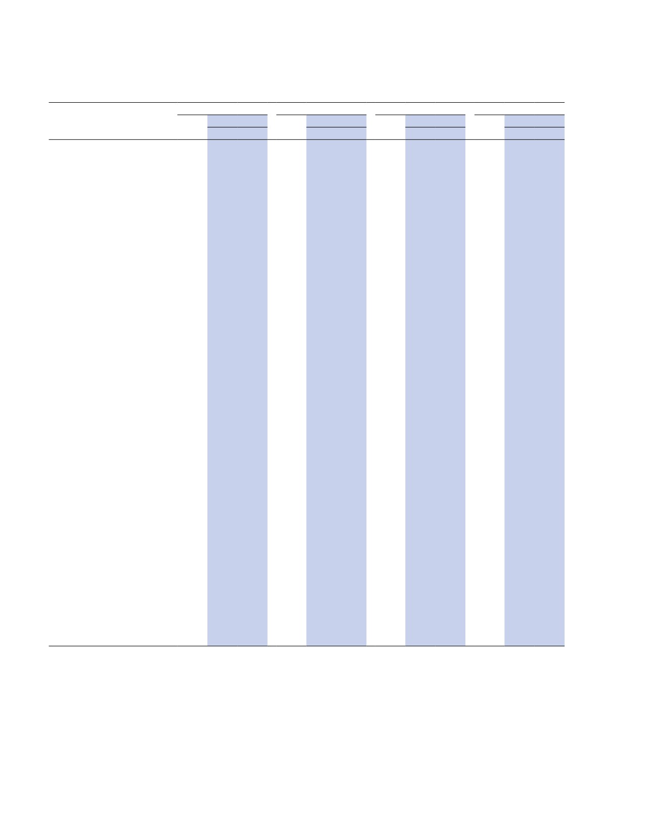
Annex Table 1.1.1. European Economies: Real GDP, Consumer Prices, Current Account Balance, and Unemployment

(Annual percent change, unless noted otherwise)

Real GDP

Consumer Prices¹

Current Account Balance²

Unemployment³

Projections

2022

2023

2024

2022

2023

2024

2022

2023

2024

2022

2023

2024

Europe

2.7

1.2

1.5

15.4

10.5

9.4

2.0

2.1

Advanced Europe

3.5

0.7

1.2

8.5

5.9

3.3

1.9

2.5

2.6

6.0

Euro Area^4,5

3.3

0.7

1.2

8.4

5.6

3.3

-0.7

1.2

1.4

6.7

6.6

6.5

Germany

1.8

-0.5

0.9

8.7

6.3

3.5

4.2

6.0

6.6

3.1

3.3

France

2.5

1.0

1.3

5.9

5.6

2.5

-2.0

-1.2

-1.3

7.3

7.4

7.3

Italy⁶

3.7

0.7

8.7

6.0

2.6

-1.2

0.7

0.9

8.1

7.9

8.0

Spain

5.8

2.5

1.7

8.3

3.5

3.9

0.6

2.1

2.0

12.9

11.8

11.3

The Netherlands

4.3

0.6

1.1

11.6

4.0

4.2

9.2

7.6

3.5

3.7

4.1

Belgium

3.2

1.0

0.9

10.3

2.5

4.3

-3.6

-2.7

-1.9

5.6

5.7

Ireland

9.4

2.0

3.3

8.1

5.2

3.0

10.8

7.8

7.2

4.5

4.1

4.2

Austria

4.8

0.1

0.8

8.6

7.8

3.7

0.7

0.1

0.0

4.8

5.1

5.4

Portugal

6.7

2.3

1.5

8.1

5.3

3.4

-1.2

1.3

1.1

6.1

6.6

6.5

Greece

5.9

2.5

2.0

9.3

4.1

2.8

-10.1

-6.9

-6.0

12.4

10.8

9.3

Finland

1.6

-0.1

1.0

7.2

4.5

1.9

-3.6

-1.7

-0.9

6.8

7.3

7.4

Slovak Republic

1.7

1.3

2.5

12.1

10.9

4.8

-8.2

-2.7

-4.0

6.2

6.1

5.9

Croatia

6.2

2.7

2.6

10.7

8.6

4.2

-1.6

-0.2

-0.4

6.8

6.3

5.9

Lithuania

1.9

-0.2

2.7

18.9

9.3

3.9

-5.1

0.0

0.9

5.9

6.5

6.3

Slovenia

2.5

2.0

2.2

8.8

7.4

4.2

-1.0

4.4

3.8

4.0

3.6

3.8

Luxembourg

1.4

-0.4

1.5

8.1

3.2

3.3

3.6

3.7

4.0

4.8

5.2

5.8

Latvia

2.8

0.5

2.6

17.2

9.9

4.2

-4.7

-3.0

-2.4

6.9

6.7

6.6

Estonia

-0.5

-2.3

2.4

19.4

10.0

3.8

-2.9

1.8

2.6

5.6

6.7

7.1

Cyprus

5.6

2.2

2.7

8.1

3.5

2.4

-9.1

-8.6

-7.9

6.8

6.7

6.4

Malta

6.9

3.8

3.3

6.1

5.8

3.1

-5.7

-3.0

-2.9

2.9

3.1

3.2

United Kingdom⁶

4.1

0.5

0.6

9.1

7.7

3.7

-3.8

-3.7

3.7

4.2

4.6

Switzerland

2.7

0.9

1.8

2.8

2.2

2.0

10.2

8.0

2.2

2.1

2.3

Sweden

2.8

-0.7

0.6

8.1

6.9

3.6

4.8

5.4

7.5

8.1

Czech Republic

2.3

0.2

2.3

15.1

10.9

4.6

-6.1

0.5

1.7

2.1

2.8

2.6

Norway

3.3

2.3

1.5

5.8

3.7

30.2

26.2

25.4

3.3

3.6

3.8

Denmark

2.7

1.7

1.4

8.5

4.2

2.8

13.5

11.4

9.9

4.5

5.0

Iceland

7.2

3.3

1.7

8.3

8.6

4.5

-2.0

-0.6

-0.4

3.8

3.4

3.8

Andorra

8.8

2.1

1.5

6.2

5.2

3.5

17.0

17.9

18.4

2.1

1.9

1.7

San Marino

5.0

2.2

1.3

5.3

5.9

2.5

8.0

3.8

2.9

4.3

4.0

3.9

Emerging and Developing Europe

0.8

2.4

2.2

27.9

18.9

19.9

2.6

-0.4

-0.3

Russia

-2.1

2.2

1.1

13.8

5.3

6.3

10.5

3.4

4.0

3.9

3.3

3.1

Türkiye⁶

5.5

4.0

3.0

72.3

51.2

62.5

-5.3

-4.2

-3.0

10.3

9.9

10.1

Poland

5.1

0.6

2.3

14.4

12.0

6.4

-3.0

1.0

0.3

2.9

2.8

2.9

Romania

4.7

2.2

3.8

13.8

10.7

5.8

-9.3

-7.3

-7.1

5.6

5.4

Ukraine⁶

-29.1

2.0

3.2

20.2

17.7

13.0

5.0

-5.7

-7.2

24.5

19.4

10.6

Hungary

4.6

-0.3

3.1

14.5

17.7

6.6

-8.0

-0.9

-1.6

3.6

3.9

3.8

Belarus

-3.7

1.6

1.3

15.2

4.7

5.7

3.7

2.7

2.0

4.2

4.0

3.6

Bulgaria

3.4

1.7

3.2

13.0

8.5

3.0

-0.7

0.0

0.1

4.2

4.6

4.4

Serbia

2.3

2.0

3.0

12.0

12.4

5.3

-6.9

-2.3

-3.2

9.4

9.1

9.0

Source: IMF staff estimates.

Note: Data for some countries are based on fiscal years. Please refer to Table F in the Statistical Appendix for a list of economies with exceptional reporting periods.

¹Movements in consumer prices are shown as annual averages. Year-end to year-end changes can be found in Tables A6 and A7 in the Statistical Appendix.

²Percent of GDP.

³Percent. National definitions of unemployment may differ.

⁴Current account position corrected for reporting discrepancies in intra-area transactions.

⁵Based on Eurostat’s harmonized index of consumer prices, except in the case of Slovenia.

⁶See the country-specific notes for Italy, Türkiye, Ukraine, and the United Kingdom in the “Country Notes” section of the Statistical Appendix.

⁷Includes Albania, Bosnia and Herzegovina, Kosovo, Moldova, Montenegro, and North Macedonia.

International Monetary Fund | October 2023

CHAPTER 1 Global Prospects and Policies

Annex Table 1.1.2. Asian and Pacific Economies: Real GDP, Consumer Prices, Current Account Balance, and Unemployment

(Annual percent change, unless noted otherwise)

Real GDP

Consumer Prices¹

Current Account Balance²

Unemployment³

Projections

2022

2023

2024

2022

2023

2024

2022

2023

2024

2022

2023

2024

Asia

3.9

4.6

4.2

3.8

2.8

2.7

1.8

1.6

1.5

Advanced Asia

1.8

2.1

1.8

3.8

3.5

2.7

3.6

3.8

3.9

2.9

2.8

2.9

Japan

1.0

2.0

1.0

2.5

3.2

2.9

2.1

3.3

3.7

2.6

2.5

2.3

Korea

2.6

1.4

2.2

5.1

3.4

2.3

1.8

1.3

1.7

2.9

2.7

3.2

Taiwan Province of China

2.4

0.8

3.0

2.9

2.1

1.5

13.3

11.8

12.1

3.7

Australia

3.7

1.8

1.2

6.6

5.8

4.0

1.1

0.6

-0.7

3.7

4.3

Singapore

3.6

1.0

2.1

6.1

5.5

3.5

19.3

16.6

15.2

2.1

1.8

Hong Kong SAR

-3.5

4.4

2.9

1.9

2.2

2.3

10.6

7.1

6.3

4.3

3.2

3.1

New Zealand

2.7

1.1

1.0

7.2

4.9

2.7

-9.0

-7.9

-6.5

3.3

3.8

4.9

Macao SAR

-26.8

74.4

27.2

1.0

0.9

1.7

-23.5

19.9

32.4

3.0

2.7

2.5

Emerging and Developing Asia

4.5

5.2

4.8

3.8

2.6

2.7

1.2

0.7

0.6

China

3.0

5.0

4.2

1.9

0.7

1.7

2.2

1.5

1.4

5.5

5.3

5.2

India⁴

7.2

6.3

6.7

5.5

4.6

-2.0

-1.8

Indonesia

5.3

5.0

4.2

3.6

2.5

1.0

-0.3

-0.6

5.9

5.3

5.2

Thailand

2.6

2.7

3.2

6.1

1.5

1.6

-3.0

-0.2

1.9

1.3

1.2

1.1

Vietnam

8.0

4.7

5.8

3.2

3.4

-0.3

0.2

0.7

2.3

2.1

Philippines

7.6

5.3

5.9

5.8

3.2

-4.5

-3.0

-2.6

5.4

4.7

5.1

Malaysia

8.7

4.0

4.3

3.4

2.9

2.7

3.1

2.7

2.8

3.8

3.6

3.5

Other Emerging and Developing Asia⁵

3.9

3.8

5.6

12.3

10.8

7.4

-3.8

-1.2

Memorandum

ASEAN-5⁶

5.5

4.2

4.5

4.8

3.6

2.5

2.7

2.3

Emerging Asia⁷

4.5

5.2

4.8

3.4

2.3

2.5

1.3

0.8

0.7

Source: IMF staff estimates.

Note: Data for some countries are based on fiscal years. Please refer to Table F in the Statistical Appendix for a list of economies with exceptional reporting periods.

¹Movements in consumer prices are shown as annual averages. Year-end to year-end changes can be found in Tables A6 and A7 in the Statistical Appendix.

²Percent of GDP.

³Percent. National definitions of unemployment may differ.

⁴See the country-specific note for India in the “Country Notes” section of the Statistical Appendix.

⁵Other Emerging and Developing Asia comprises Bangladesh, Bhutan, Brunei Darussalam, Cambodia, Fiji, Kiribati, Lao P.D.R., Maldives, the Marshall Islands, Micronesia,

Mongolia, Myanmar, Nauru, Nepal, Palau, Papua New Guinea, Samoa, the Solomon Islands, Sri Lanka, Timor-Leste, Tonga, Tuvalu, and Vanuatu.

⁶Indonesia, Malaysia, the Philippines, Singapore, and Thailand.

⁷Emerging Asia comprises China, India, Indonesia, Malaysia, the Philippines, Thailand, and Vietnam.

International Monetary Fund | October 2023

WORLD ECONOMIC OUTLOOK: Navigating Global Divergences

Annex Table 1.1.3. Western Hemisphere Economies: Real GDP, Consumer Prices, Current Account Balance, and Unemployment

(Annual percent change, unless noted otherwise)

Real GDP

Consumer Prices¹

Current Account Balance²

Unemployment³

Projections

2022

2023

2024

2022

2023

2024

2022

2023

2024

2022

2023

2024

North America

2.3

2.1

1.5

7.9

4.2

2.8

-3.4

-2.7

-2.6

United States

2.1

1.5

8.0

4.1

2.8

-3.8

-3.0

-2.8

3.6

3.8

Mexico

3.9

3.2

2.1

7.9

5.5

3.8

-1.2

-1.5

-1.4

3.3

2.9

3.1

Canada

3.4

1.3

1.6

6.8

3.6

2.4

-0.3

-1.0

5.3

5.5

6.3

Puerto Rico⁴

2.0

-0.7

-0.2

5.9

2.9

1.5

6.2

6.8

6.6

South America⁵

3.8

1.6

2.0

17.4

18.7

14.7

-3.0

-1.9

-1.6

Brazil

2.9

3.1

1.5

9.3

4.7

4.5

-2.8

-1.9

-1.8

9.3

8.3

8.2

Argentina

5.0

-2.5

2.8

72.4

121.7

93.7

-0.7

-0.6

1.2

6.8

7.4

7.2

Colombia

7.3

1.4

2.0

10.2

11.4

5.2

-6.2

-4.9

-4.3

11.2

10.8

10.4

Chile

2.4

-0.5

1.6

11.6

7.8

3.6

-9.0

-3.5

-3.6

7.9

8.8

9.0

Peru

2.7

1.1

2.7

7.9

6.5

2.9

-4.1

-1.9

-2.1

7.8

7.6

7.4

Ecuador

2.9

1.4

1.8

3.5

2.3

1.8

2.4

1.5

1.6

3.2

3.8

3.9

Venezuela

8.0

4.0

4.5

186.5

360.0

200.0

3.6

2.2

3.4

Bolivia

3.5

1.8

1.7

3.0

4.4

-0.4

-2.7

-3.3

4.7

4.9

5.0

Paraguay

0.1

4.5

3.8

9.8

4.7

4.1

-6.0

0.6

0.1

6.8

6.2

6.0

Uruguay

4.9

1.0

3.2

9.1

6.1

5.9

-3.5

-3.7

-3.3

7.9

8.1

8.0

Central America⁶

5.4

3.8

3.9

7.2

4.2

3.6

-3.2

-2.2

-2.1

Caribbean⁷

13.9

9.8

8.3

12.6

13.2

6.5

4.4

0.8

2.0

Memorandum

Latin America and the Caribbean⁸

4.1

2.3

14.0

13.8

10.7

-2.4

-1.8

-1.5

Eastern Caribbean Currency Union⁹

9.9

4.7

4.0

5.5

4.2

2.4

-13.4

-11.3

-10.2

Source: IMF staff estimates.

Note: Data for some countries are based on fiscal years. Please refer to Table F in the Statistical Appendix for a list of economies with exceptional reporting periods.

¹Movements in consumer prices are shown as annual averages. Year-end to year-end changes can be found in Tables A6 and A7 in the Statistical Appendix. Aggregates exclude

Venezuela.

²Percent of GDP.

³Percent. National definitions of unemployment may differ.

⁴Puerto Rico is a territory of the United States, but its statistical data are maintained on a separate and independent basis.

⁵See the country-specific notes for Argentina and Venezuela in the “Country Notes” section of the Statistical Appendix.

⁶Central America refers to CAPDR (Central America, Panama, and the Dominican Republic) and comprises Costa Rica, the Dominican Republic, El Salvador, Guatemala,

Honduras, Nicaragua, and Panama.

⁷The Caribbean comprises Antigua and Barbuda, Aruba, The Bahamas, Barbados, Belize, Dominica, Grenada, Guyana, Haiti, Jamaica, St. Kitts and Nevis, St. Lucia, St. Vincent

and the Grenadines, Suriname, and Trinidad and Tobago.

⁸Latin America and the Caribbean comprises Mexico and economies from the Caribbean, Central America, and South America. See the country-specific notes for Argentina and

Venezuela in the “Country Notes” section of the Statistical Appendix.

⁹Eastern Caribbean Currency Union comprises Antigua and Barbuda, Dominica, Grenada, St. Kitts and Nevis, St. Lucia, and St. Vincent and the Grenadines, as well as Anguilla

and Montserrat, which are not IMF members.

International Monetary Fund | October 2023

CHAPTER 1 Global Prospects and Policies

Annex Table 1.1.4. Middle East and Central Asia Economies: Real GDP, Consumer Prices, Current Account Balance, and

Unemployment

(Annual percent change, unless noted otherwise)

Real GDP

Consumer Prices¹

Current Account Balance²

Unemployment³

Projections

2022

2023

2024

2022

2023

2024

2022

2023

2024

2022

2023

2024

Middle East and Central Asia

5.6

2.0

3.4

14.0

18.0

15.2

8.6

4.1

3.6

Oil Exporters⁴

5.7

2.2

3.4

13.3

12.9

9.4

13.8

6.8

6.0

Saudi Arabia

8.7

0.8

4.0

2.5

2.2

13.6

5.9

5.4

5.6

Iran

3.8

3.0

2.5

45.8

47.0

32.5

4.2

3.4

3.7

9.3

9.4

9.6

United Arab Emirates

7.9

3.4

4.0

4.8

3.1

2.3

11.7

8.2

7.7

Kazakhstan

3.3

4.6

4.2

15.0

9.0

3.5

-1.5

-0.7

4.9

4.8

Algeria

3.2

3.8

3.1

9.3

9.0

6.8

9.8

2.9

1.0

Iraq

7.0

-2.7

2.9

5.0

5.3

3.6

17.3

-1.9

-4.3

Qatar

4.9

2.4

2.2

5.0

2.8

2.3

26.7

17.6

15.4

Kuwait

8.9

-0.6

3.6

4.0

3.4

3.1

36.0

30.3

27.7

2.2

Azerbaijan

4.6

2.5

13.9

10.3

5.6

29.8

16.3

15.7

5.9

5.8

Oman

4.3

1.2

2.7

2.8

1.1

1.7

6.4

5.1

5.4

Turkmenistan

1.6

2.5

2.1

11.2

5.9

10.5

7.1

3.4

1.8

Bahrain

4.9

2.7

3.6

1.0

1.4

15.4

6.6

7.0

5.4

Oil Importers^5,6

5.3

1.8

3.3

15.1

26.7

25.1

-5.1

-3.1

-3.6

Egypt

6.7

4.2

3.6

8.5

23.5

32.2

-3.5

-1.7

-2.4

7.3

7.1

7.5

Pakistan

6.1

-0.5

2.5

12.1

29.2

23.6

-4.7

-0.7

-1.8

6.2

8.5

8.0

Morocco

1.3

2.4

3.6

6.6

6.3

3.5

-3.5

-3.1

-3.2

11.8

12.0

11.7

Uzbekistan

5.7

5.5

11.4

10.2

10.0

-0.8

-4.3

-4.6

8.9

8.4

7.9

Sudan⁷

-2.5

-18.3

0.3

138.8

256.2

152.4

-11.2

-1.0

-7.4

32.1

46.0

47.2

Tunisia

2.5

1.3

1.9

8.3

9.4

9.8

-8.6

-5.8

-5.4

15.2

Jordan

2.5

2.6

2.7

4.2

2.7

2.6

-8.8

-7.6

-5.4

22.9

Georgia

10.1

6.2

4.8

11.9

2.4

2.7

-4.0

-6.1

-5.8

17.3

18.4

18.6

Armenia

12.6

7.0

5.0

8.6

3.5

4.0

0.8

-1.4

-2.3

13.0

13.5

14.0

Tajikistan

8.0

6.5

5.0

6.6

4.6

5.7

15.6

-3.7

-2.4

Kyrgyz Republic

6.3

3.4

4.3

13.9

11.7

8.6

-46.5

-20.0

-6.1

9.0

West Bank and Gaza⁷

3.9

3.0

2.7

3.7

3.4

2.7

24.4

24.2

24.0

Mauritania

6.5

4.5

5.3

9.6

7.5

4.0

-15.3

-9.9

-11.1

Memorandum

Caucasus and Central Asia

4.8

4.6

4.2

13.0

11.0

8.3

6.0

0.4

0.6

Middle East, North Africa, Afghanistan,

5.7

1.7

3.3

14.1

19.0

16.2

8.9

4.7

4.0

and Pakistan⁶

Middle East and North Africa

5.6

2.0

3.4

14.4

17.5

15.0

10.2

5.2

4.6

Israel⁸

6.5

3.1

3.0

4.4

4.3

3.0

3.4

4.2

4.0

3.8

3.5

3.9

Source: IMF staff estimates.

Note: Data for some countries are based on fiscal years. Please refer to Table F in the Statistical Appendix for a list of economies with exceptional reporting periods.

¹Movements in consumer prices are shown as annual averages. Year-end to year-end changes can be found in Tables A6 and A7 in the Statistical Appendix.

²Percent of GDP.

³Percent. National definitions of unemployment may differ.

⁴Includes Libya and Yemen.

⁵Includes Djibouti, Lebanon, and Somalia. See the country-specific note for Lebanon in the “Country Notes” section of the Statistical Appendix.

⁶Excludes Afghanistan and Syria because of the uncertain political situation. See the country-specific notes in the “Country Notes” section of the Statistical Appendix.

⁷See the country-specific notes for Sudan and West Bank and Gaza in the “Country Notes” section of the Statistical Appendix.

⁸Israel, which is not a member of the economic region, is shown for reasons of geography but is not included in the regional aggregates.

International Monetary Fund | October 2023

WORLD ECONOMIC OUTLOOK: Navigating Global Divergences

Annex Table 1.1.5. Sub-Saharan African Economies: Real GDP, Consumer Prices, Current Account Balance, and Unemployment

(Annual percent change, unless noted otherwise)

Real GDP

Consumer Prices¹

Current Account Balance²

Unemployment³

Projections

2022

2023

2024

2022

2023

2024

2022

2023

2024

2022

2023

2024

Sub-Saharan Africa

4.0

3.3

4.0

14.5

15.8

13.1

-1.9

-2.7

-2.8

Oil Exporters⁴

3.2

2.5

3.0

18.0

21.6

21.3

2.8

1.1

0.9

Nigeria

3.3

2.9

3.1

18.8

25.1

23.0

0.2

0.7

0.6

Angola

3.0

1.3

3.3

21.4

13.1

22.3

9.6

3.1

3.7

Gabon

3.0

2.8

2.6

4.3

3.8

2.5

1.6

-0.8

-2.1

Chad

3.4

4.0

3.7

5.8

7.0

3.5

6.2

0.2

-3.3

Equatorial Guinea

3.2

-6.2

-5.5

4.9

2.4

4.0

9.6

-2.6

-3.0

Middle-Income Countries⁵

3.6

2.7

3.6

9.4

6.6

-2.7

-3.3

-3.0

South Africa

1.9

0.9

1.8

6.9

5.8

4.8

-0.5

-2.5

-2.8

33.5

32.8

Kenya

4.8

5.0

5.3

7.6

7.7

6.6

-5.1

-4.9

Ghana

3.1

1.2

2.7

31.9

42.2

23.2

-2.1

-2.5

-2.8

Côte d'Ivoire

6.7

6.2

6.6

5.2

4.3

2.3

-6.5

-4.7

-3.8

Cameroon

3.8

4.0

4.2

6.3

7.2

4.8

-1.8

-2.6

-2.4

Zambia

4.7

3.6

4.3

11.0

10.6

9.6

3.6

5.0

7.4

Senegal

4.0

4.1

8.8

9.7

6.1

3.3

-19.9

-14.6

-7.9

Low-Income Countries⁶

5.7

5.3

5.8

18.7

19.1

14.1

-6.8

-5.5

-5.7

Ethiopia

6.4

6.1

6.2

33.9

29.1

20.7

-4.3

-2.4

-2.0

Tanzania

4.7

5.2

6.1

4.4

4.0

-5.4

-5.1

-4.2

Democratic Republic of the Congo

8.9

6.7

4.7

9.3

19.1

10.6

-5.2

-6.0

-5.3

Uganda

6.4

4.6

5.7

7.2

5.8

4.7

-8.2

-7.1

-8.2

Burkina Faso

1.5

4.4

6.4

14.1

1.4

3.0

-6.2

-5.1

-5.2

Mali

3.7

4.5

4.8

9.7

5.0

2.8

-6.9

-6.5

-5.7

Source: IMF staff estimates.

Note: Data for some countries are based on fiscal years. Please refer to Table F in the Statistical Appendix for a list of economies with exceptional reporting periods.

¹Movements in consumer prices are shown as annual averages. Year-end to year-end changes can be found in Tables A6 and A7 in the Statistical Appendix.

²Percent of GDP.

³Percent. National definitions of unemployment may differ.

⁴Includes Republic of Congo and South Sudan.

⁵Includes Benin, Botswana, Cabo Verde, the Comoros, Eswatini, Lesotho, Mauritius, Namibia, São Tomé and Príncipe, and Seychelles.

⁶Includes Burundi, Central African Republic, Eritrea, The Gambia, Guinea, Guinea-Bissau, Liberia, Madagascar, Malawi, Mozambique, Niger, Rwanda, Sierra Leone, Togo, and

Zimbabwe.

International Monetary Fund | October 2023

CHAPTER 1

Global Prospects and Policies

Annex Table 1.1.6. Summary of World Real per Capita Output

(Annual percent change; in constant 2017 international dollars at purchasing power parity)

Average

Projections

2005-14

2015

2016

2017

2018

2019

2020

2021

2022

2023

2024

World

2.3

2.0

1.9

2.5

1.7

-4.0

5.3

3.0

2.0

1.9

Advanced Economies

0.9

1.7

1.3

2.1

1.9

1.3

-4.7

5.5

2.2

1.1

United States

0.8

2.0

0.9

1.6

2.4

1.8

-3.6

5.6

1.7

1.6

1.0

Euro Area¹

0.4

1.7

1.6

2.5

1.6

1.4

-6.4

5.8

3.2

0.5

1.1

Germany

1.4

0.6

1.4

2.3

0.7

0.8

-3.9

3.1

1.1

-0.6

0.9

France

0.4

0.6

0.7

2.2

1.5

-7.9

6.1

2.2

0.7

1.1

Italy²

-0.9

0.9

1.5

1.8

1.1

0.7

-8.7

7.7

4.1

1.0

Spain

-0.4

3.9

2.9

2.8

1.9

1.2

-11.6

6.5

5.1

2.0

1.3

Japan

0.6

1.7

0.8

1.8

0.8

-0.2

-4.0

2.5

1.3

2.4

1.5

United Kingdom²

0.5

1.6

1.3

1.8

1.1

-11.4

7.3

3.3

0.0

0.2

Canada

0.9

-0.1

0.0

1.8

1.4

0.4

-6.2

4.4

1.7

-1.1

0.2

Other Advanced Economies³

2.3

1.5

1.8

2.4

2.0

1.2

-2.2

5.8

1.8

1.0

1.6

Emerging Market and Developing Economies

4.3

2.8

3.3

2.3

-3.1

5.7

3.5

2.9

Emerging and Developing Asia

7.1

5.8

5.7

5.6

4.4

-1.3

6.7

3.9

4.6

4.2

China

9.4

6.5

6.2

6.4

6.3

5.6

2.1

8.4

3.1

5.0

4.2

India²

6.2

6.7

7.0

5.6

5.3

2.8

-6.7

8.2

6.5

5.5

5.3

Emerging and Developing Europe

3.5

0.5

1.5

4.0

3.4

2.3

-1.5

7.4

2.7

1.9

Russia

3.3

-2.2

0.0

1.8

2.9

2.2

-2.3

6.1

-0.6

2.4

1.3

Latin America and the Caribbean

2.2

-0.8

-1.9

0.3

0.2

-1.0

-8.1

6.4

3.3

1.5

1.4

Brazil

2.6

-4.1

-3.8

0.8

1.3

0.7

-3.7

4.4

2.4

2.5

0.9

Mexico

0.4

1.5

0.6

0.8

0.9

-1.3

-9.5

4.9

3.0

2.3

1.3

Middle East and Central Asia

1.8

0.6

2.0

0.0

0.7

-0.2

-4.7

2.4

7.2

0.1

1.6

Saudi Arabia

0.7

-0.6

-1.4

-0.1

5.4

1.3

-8.9

6.5

4.0

-1.2

1.9

Sub-Saharan Africa

2.5

0.4

-1.3

0.2

0.5

0.4

-4.3

2.1

1.4

0.8

1.4

Nigeria

4.1

0.0

-4.2

-1.8

-0.7

-0.4

-4.3

1.1

0.7

0.4

0.6

South Africa

1.6

-0.2

-0.8

-0.3

0.1

-1.2

-7.3

3.8

1.1

-0.6

0.3

Memorandum

European Union

0.8

2.1

1.8

2.9

2.1

1.8

-5.8

6.0

3.4

0.5

1.3

ASEAN-5⁴

3.7

3.3

3.6

4.1

3.9

3.2

-5.4

3.2

4.5

3.2

3.6

Middle East and North Africa

1.3

0.4

2.3

-0.7

0.4

-0.7

-5.2

2.5

3.5

0.1

1.6

Emerging Market and Middle-Income Economies

4.6

3.0

3.1

3.6

2.5

-3.0

6.4

3.4

3.3

3.1

Low-Income Developing Countries

3.5

2.2

1.5

2.5

2.7

2.6

-1.2

1.1

4.1

1.6

2.9

Source: IMF staff estimates.

Note: Data for some countries are based on fiscal years. Please refer to Table F in the Statistical Appendix for a list of economies with exceptional reporting periods.

¹Data are calculated as the sum of those for individual euro area countries.

²See the country-specific notes for India, Italy, and the United Kingdom in the “Country Notes” section of the Statistical Appendix.

³Excludes the Group of Seven (Canada, France, Germany, Italy, Japan, United Kingdom, United States) and euro area countries.

⁴ASEAN-5 comprises Indonesia, Malaysia, the Philippines, Singapore, and Thailand.

International Monetary Fund | October 2023

WORLD ECONOMIC OUTLOOK: Navigating Global Divergences

References

Brookings Papers on Economic Activity 1: 91-142. https://www

Abdelrahman, Hamza, and Luiz E. Oliveira. 2023. “Te Rise

.brookings.edu/wp-content/uploads/1997/01/1997a_bpea

and Fall of Pandemic Excess Savings.” FRBSF Economic

_bernanke_gertler_watson_sims_friedman.pdf.

Letter 2023-11, Federal Reserve Bank of San Francisco,

Blanchard, Olivier, and Ben S. Bernanke. 2023. “What Caused

San Francisco.

the US Pandemic-Era Inflation?” NBER Working Paper

Abiad, Abdul, Ravi Balakrishnan, Petya Koeva Brooks, Ðaniel Leigh,

31417, National Bureau of Economic Research, Cambridge,

and Irina Tytell. 2009. “What’s the Damage? Medium-Term

MA. https://www.nber.org/papers/w31417.

Output Dynamics after Banking Crises.” IMF Working Paper

Bloom, Nicholas, Charles I. Jones, John Van Reenen, and

09/245, International Monetary Fund, Washington, DC.

Michael Webb. 2020. “Are Ideas Getting Harder to Find?”

Acemoglu, Daron, David Autor, and Christina Patterson. 2023.

American Economic Review 110 (4): 1104-44.

“Bottlenecks: Sectoral Imbalances and the US Productivity

Brasili, Andrea, Cristina Brasili, Giorgio Musto, and Anamaria

Slowdown.” NBER Working Paper 31427, National Bureau

Tüske. 2023. “Complementarities between Local Public and

of Economic Research, Cambridge, MA.

Private Investment in EU Regions.” European Investment

Adrian, Tobias, Gita Gopinath, and Pierre-Olivier Gourinchas.

Bank Working Paper 2023/04, Luxembourg.

2023. “Central Banks Can Fend Off Financial Turmoil and

Breitenlechner, Max, Georgios Georgiadis, and Ben Schumann.

Still Fight Inflation.” IMF Blog, June 23.

2022. “What Goes around Comes around: How Large Are

Adrian, Tobias, Fabio Natalucci, and Jason Wu. 2023. “Inflation

Spillbacks from US Monetary Policy?” Journal of Monetary

Remains Risk Confronting Financial Markets.” IMF Blog,

Economics 131 (2022): 45-60.

July 27. https://www.imf.org/en/Blogs/Articles/2023/07/27/

Bruno, Valentina, and Hyun Song Shin. 2015. “Capital Flows

inflation-remains-risk-confronting-financial-markets.

and the Risk-Taking Channel of Monetary Policy.” Journal

Aiyar, Shekhar, Jiaqian Chen, Christian Ebeke, Roberto

of Monetary Economics 71: 119-32. https://doi.org/10.1016/j

Garcia-Saltos, Tryggvi Gudmundsson, Anna Ilyina, Alvar

.jmoneco.2014.11.011.

Kangur, and others. 2023. “Geoeconomic Fragmentation and

Brussevich, Maria, Shihui Liu, and Chris Papageorgiou. 2022.

the Future of Multilateralism.” IMF Staff Discussion Note

“Income Convergence or Divergence in the Aftermath of the

23/001, International Monetary Fund, Washington, DC.

COVID-19 Shock?” IMF Working Paper 22/121, Interna-

https://www.imf.org/en/Publications/Staff-Discussion-Notes/

tional Monetary Fund, Washington, DC.

Issues/2023/01/11/Geo-Economic-Fragmentation-and-the

Budina, Nina, Christian Ebeke, Florence Jaumotte, Andrea

-Future-of-Multilateralism-527266.

Medici, Augustus J. Panton, Marina M. Tavares, and Bella Yao.

Andrle, Michal, Patrick Blagrave, Pedro Espaillat, Keiko Honjo,

2023. “Structural Reforms to Accelerate Growth, Ease Policy

Benjamin Hunt, Mika Kortelainen, René Lalonde, and others.

Trade-Offs, and Support the Green Transition in EMDEs.”

2015. “Te Flexible System of Global Models—FSGM.” IMF

Unpublished, International Monetary Fund, Washington, DC.

Working Paper 15/64, International Monetary Fund, Washing-

Capelle, Damien, Divya Kirti, Nicola Pierri, and German

ton, DC. https://www.imf .org/en/Publications/WP/Issues/

Villegas Bauer. Forthcoming. “Mitigating Climate Change

2016/12/31/Te-Flexible-System-of-Global-Models-FSGM-

at the Firm Level: Mind the Laggards.” IMF Working Paper,

42796.

International Monetary Fund, Washington, DC.

Andrle, Michal, and Benjamin Hunt. 2020. “Model-Based

Colonna, Fabrizio, Roberto Torrini, and Eliana Viviano. 2023. “Te

Globally-Consistent Risk Assessment.” IMF Working Paper

Profit Share and Firm Mark-Up: How to Interpret Tem?” Bank

20/64, International Monetary Fund, Washington, DC.

of Italy Occasional Papers 770, Bank of Italy, Rome. https://www

https://www.imf.org/en/Publications/WP/Issues/2020/05/22/

.bancaditalia.it/pubblicazioni/qef/2023-0770/.

Model-Based-Globally-Consistent-Risk-Assessment-49253.

Dao, Mai Chi, Allan Dizioli, Chris Jackson, Pierre-Olivier

Ball, Laurence M., Daniel Leigh, and Prachi Mishra. 2022.

Gourinchas, and Daniel Leigh. 2023. “Unconventional Fiscal

“Understanding U.S. Inflation during the COVID-19

Policy in Times of High Inflation.” IMF Working Paper 23/178,

Era.” Brookings Papers on Economic Activity (Fall): 1-54.

International Monetary Fund, Washington, DC. https://www

https://www.brookings.edu/projects/brookings-papers-on

.imf.org/en/Publications/WP/Issues/2023/08/31/Unconventional

-economic-activity.

-Fiscal-Policy-in-Times-of-High-Inflation-537454.

Baqaee, David Rezza, and Emmanuel Farhi. 2020. “Productivity

de Soyres, Francois, Dylan Moore, and Julio L. Ortiz. 2023.

and Misallocation in General Equilibrium.” Quarterly Journal

“Accumulated Savings during the Pandemic: An International

of Economics 135 (1): 105-63.

Comparison with Historical Perspective.” FEDS Notes. Board

Barrett, Philip, Maximiliano Appendino, Kate Nguyen, and

of Governors of the Federal Reserve System, June 23. https://

Jorge de Lion Miranda. 2022. “Measuring Social Unrest

doi.org/10.17016/2380-7172.3326.

Using Media Reports.” Journal of Development Economics 158:

Dées, Stéphane, and Alessandro Galesi. 2021. “Te Global

102924. https://doi.org/10.1016/j.jdeveco.2022.102924.

Financial Cycle and US Monetary Policy in an Interconnected

Bernanke, Ben S., Mark Gertler, and Mark Watson. 1997. “Sys-

World.” Journal of International Money and Finance 115:

tematic Monetary Policy and the Effects of Oil Price Shocks.”

102395. https://doi.org/10.1016/j.jimonfin.2021.102395.

International Monetary Fund | October 2023

CHAPTER 1 Global Prospects and Policies

Food and Agriculture Organization (FAO), International Fund for

Kearns, Jonathan, Andreas Schrimpf, and Fan Dora Xia. 2023.

Agricultural Development, United Nations Children’s Fund,

“Explaining Monetary Spillovers: Te Matrix Reloaded.” Jour-

World Food Programme, and World Health Organization.

nal of Money, Credit and Banking 55 (6): 1535-68. https://doi

2023. “In Brief: Te State of Food Security and Nutrition in

.org/10.1111/jmcb.12996.

the World 2023: Urbanization, Agrifood Systems Transforma-

Kilic Celik, Sinem, M. Ayhan Kose, and Franziska Ohnsorge.

tion and Healthy Diets across the Rural-Urban Continuum.”

2023. “Potential Growth Prospects: Risks, Rewards, and

Rome. https://www.fao.org/documents/card/en/c/cc6550en.

Policies.” Policy Research Working Paper 10355, World Bank,

Gagliardone, Luca, and Mark Gertler. 2023. “Oil Prices, Mon-

Washington, DC.

etary Policy and Inflation Surges.” NBER Working Paper

Mahler, Daniel Gerszon, Nishant Yonzan, Ruth Hill,

31263, National Bureau of Economic Research, Cambridge,

Christopher Lakner, Haoyu Wu, and Nobuo Yoshida. 2022.

MA. https://www.nber.org/papers/w31263.

“Pandemic, Prices, and Poverty.” Data Blog (World Bank),

Gertler, Mark, and Peter Karadi. 2015. “Monetary Policy

April 13. https://blogs.worldbank.org/opendata/pandemic

Surprises, Credit Costs, and Economic Activity.” American

-prices-and-poverty.

Economic Journal: Macroeconomics 7 (1): 44-76. https://doi

Miao, Yanliang, Weifeng Wu, and Norbert Funke. 2011. “Reviv-

.org/10.1257/mac.20130329.

ing the Competitive Storage Model: A Holistic Approach

Gourinchas, Pierre-Olivier. 2019. “Te Dollar Hegemon?

to Food Commodity Prices.” IMF Working Paper 11/64,

Evidence and Implications for Policymakers.” In Te Asian

International Monetary Fund, Washington, DC. https://www

Monetary Policy Forum: Insights for Central Banking, edited by

.imf.org/en/Publications/WP/Issues/2016/12/31/Reviving-the

Steven J. Davis, Edward S. Robinson, and Bernard Young,

-Competitive-Storage-Model-A-Holistic-Approach-to-Food

264-300. Singapore: World Scientific. https://doi.org/10

-Commodity-Prices-24720.

.1142/9789811238628_0007.

Milesi-Ferretti, Gian Maria. 2021. “Te Travel Shock.” Hutchins

Ha, Jongrim, M. Ayhan Kose, and Franziska Ohnsorge. 2021.

Center Working Paper 74, Hutchins Center on Fiscal and

“One-Stop Source: A Global Database of Inflation.” Policy

Monetary Policy, Brookings Institution, Washington, DC.

Research Working Paper 9737, World Bank, Washington,

https://www.brookings.edu/wp-content/uploads/2021/08/

DC. https://openknowledge.worldbank.org/server/api/core/

WP74-Milesi-Ferretti.pdf.

bitstreams/5a5fb3ef-6d71-58c4-a8e2-34d4804dd2e7/content.

Miranda-Agrippino, Silvia, and Hélène Rey. 2020. “US

Hadzi-Vaskov, Metodij, Samuel Pienknagura, and Luca Antonio

Monetary Policy and the Global Financial Cycle.” Review of

Ricci. 2021. “Te Macroeconomic Impact of Social Unrest.” IMF

Economic Studies 87 (6): 2754-776. https://doi.org/10.1093/

Working Paper 21/135, International Monetary Fund, Washing-

restud/rdaa019.

ton, DC. https://www.imf.org/en/Publications/WP/Issues/2021/

Miranda-Pinto, Jorge, Andrea Pescatori, Ervin Prifti, and Guill-

05/07/Te-Macroeconomic-Impact-of-Social-Unrest-50338.

ermo Verduzco Bustos. 2023. “Monetary Policy Transmission

Hofmann, Boris, Deniz Igan, and Daniel Rees. 2023. “Te

through Commodity Prices.” IMF Working Paper 23/215,

Changing Nexus between Commodity Prices and the Dollar:

International Monetary Fund, Washington, DC.

Causes and Implications.” BIS Bulletin 74, Bank for Interna-

Platzer, Josef, and Marcel Peruffo. 2022. “Secular Drivers of the

tional Settlements, Basel, Switzerland. https://www.bis.org/

Natural Rate of Interest in the United States: A Quantita-

publ/bisbull74.htm.

tive Evaluation.” IMF Working Paper 22/30, International

Ider, Gökhan, Alexander Kriwoluzky, Frederik Kurcz, and Ben

Monetary Fund, Washington, DC. https://www.imf.org/

Schumann. 2023. “Te Energy-Price Channel of (European)

en/Publications/WP/Issues/2022/02/11/Secular-Drivers

Monetary Policy.” DIW Berlin Discussion Paper 2033, Ger-

-of-the-Natural-Rate-of-Interest-in-the-United-States-A

man Institute for Economic Research, Berlin.

-Quantitative-512755.

International Labour Organization (ILO). 2023. “A Global

Rey, Hélène. 2013. “Dilemma, not Trilemma: Te Global Finan-

Employment Divide: Low-Income Countries Will Be Left

cial Cycle and Monetary Policy Independence.” In Jackson

Further behind without Action on Jobs and Social Protec-

Hole Economic Policy Proceedings, Federal Reserve Bank of

tion.” ILO Monitor on the World of Work, 11th ed. Geneva.

Kansas City, 285-333. Federal Reserve Bank of Kansas City.

https://www.ilo.org/beijing/what-we-do/publications/WCMS

https://www.kansascityfed.org/Jackson%20Hole/documents/

_883341/lang--en/index.htm.

4575/2013Rey.pdf.

International Monetary Fund (IMF). 2020. “Kurzarbeit:

Schnabel, Isabel. 2023. “Te Risks of Stubborn Inflation.”

Germany’s Short-Time Work Benefit.” IMF Blog, July 15.

Speech delivered at the Euro50 Group Conference “New

https://www.imf.org/en/News/Articles/2020/06/11/na061120

Challenges for the Economic and Monetary Union in the

-kurzarbeit-germanys-short-time-work-benefit.

Post-crisis Environment,” Luxembourg, June 19. https://

Jarociński, Marek, and Peter Karadi. 2020. “Deconstruct-

www.ecb.europa.eu/press/key/date/2023/html/ecb.sp230619

ing Monetary Policy Surprises—Te Role of Information

_1~2c0bdf2422.en.html.

Shocks.” American Economic Journal: Macroeconomics 12

Tang, Ke, and Wei Xiong. 2012. “Index Investment and the

(2): 1-43. https://www.aeaweb.org/articles?id=10.1257/

Financialization of Commodities.” Financial Analysts Journal

mac.20180090.

68 (6): 54-74. https://doi.org/10.2469/faj.v68.n6.5.

International Monetary Fund | October 2023

MANAGING EXPECTATIONS: INFLATION AND MONETARY POLICY

Inflation reached multidecade highs in many economies

Introduction

in 2022. While headline inflation has since come down

In the wake of the shocks of the COVID-19

as supply chain disruptions have eased and commodity

pandemic and Russia’s invasion of Ukraine, infla-

prices have declined, core inflation is proving stickier. The

tion around the world reached multidecade highs in

specter of high inflation becoming embedded in expecta-

2022, well above central bank targets, particularly

tions and leading to pricing choices that keep inflation

in advanced economies (see Chapter 1, Figure 1.7).

high haunts central banks. This chapter unpacks recent

As policy tightening gradually rebalances aggregate

patterns in inflation expectations and studies their role

demand toward potential output, supply chain disrup-

in driving inflation, and the implications for monetary

tions have eased, and commodity prices have declined,

policy. Expectations from professional forecasters, financial

headline inflation is coming down, but underlying

markets, and households and a new indicator for firms’

price pressures (as captured by core inflation) remain

views agree about broad inflation dynamics. Histori-

elevated. Professional forecasters expect inflation rates

cal episodes in which inflation expectations rose over a

will return closer to central banks’ targets in 2024,

sustained period of at least a year suggest that it takes

with a shift in their median deviation toward zero and

about three years for inflation and near-term (over the

a sharp narrowing of the distribution (Figure 2.1).¹

next 12 months) inflation expectations to come back to

However, they also expect that, given the current

pre-episode levels on average, given historical monetary

contractionary stance and anticipated policy action

policy reactions. Although long-term (five years in the

going forward, rates will be fully back at targets only

future) inflation expectations have generally remained

by 2026, on average.

anchored on average, near-term expectations have risen

Since consumption and investment decisions as

markedly across economies since 2022. Empirical esti-

well as price- and wage-setting processes partly reflect

mates of the expectations channel point to the growing

households’ and firms’ expectations about the future

importance of near-term expectations for understanding

pace of price changes, inflation expectations play a

inflation dynamics. Using a new macroeconomic model

critical role in shaping inflation dynamics. Amid the

with a mix of forward- and backward-looking learners,

current higher inflation environment, some observers

analysis shows how economies with greater shares of more

have expressed concerns that expectations could remain

backward-looking learners prolong price pressures and

elevated or even rise further and long-term expecta-

diminish the potency of monetary policy, since such agents

tions could de-anchor from target inflation rates. In

do not consider the future impacts of monetary policy.

turn, expectations that future inflation will rise could

The share of backward-looking learners in the economy is

feed into current inflation rates, keeping them high. If

estimated to be larger in emerging market than advanced

an expectations channel for inflation is important, it

economies. By fostering an increase in the share of

also means that policies that bring expectations down

forward-looking learners, improvements in monetary pol-

could help to lower inflation more quickly and easily.

icy frameworks and central bank communication strategies

Te idea is that the more effective monetary policy-

can help bring inflation back to target more quickly and

makers are in influencing inflation expectations, the

at a lower output cost—in other words, they can increase

lower the cost in forgone output involved in central

the chances that the economy makes a “soft landing.”

banks achieving their inflation objectives (Sargent

1983; Ball 1994). In other words, the expectations

Te authors of this chapter are Silvia Albrizio (co-lead), John

channel is critical to whether central banks can achieve

Bluedorn (co-lead), Allan Dizioli, Christoffer Koch, and Philippe

Wingender, with support from Yaniv Cohen, Pedro Simon, and Isaac

Warren. Arash Sheikholeslam and Mona Wang provided computa-

¹Professional forecasters are typically private sector forecasters

tional and technical assistance. Yuriy Gorodnichenko was an external

and do not include IMF forecasters that contribute to the World

consultant. Te chapter benefited from comments by Robert Rich

Economic Outlook forecasts. See Consensus Economics’ criteria for

and internal seminar participants and reviewers.

inclusion in their survey for further details.

International Monetary Fund | October 2023

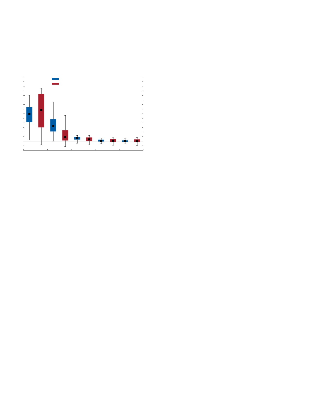
WORLD ECONOMIC OUTLOOK: Navigating Global Divergences

Figure 2.1. Cross-Economy Deviations of Inflation

influence monetary policy effectiveness and vice versa.²

Expectations from Targets

It addresses the following questions:

(Percentage points)

••

How have inflation expectations across different

agents and at alternative horizons behaved before

Inflation rates are expected to revert to targets, but only gradually over the next

two years.

and after the pandemic across economies? Are there

signs of inflation expectations deanchoring since

Advanced economies

2021? Or do the rapid interest rate hikes over 2022

Emerging market and developing economies

appear to have contained risks?

••

How important are expectations in explaining infla-

tion dynamics, particularly since the COVID-19

shock? Does the prevailing level of inflation (high

or low) affect the explanatory power of inflation

expectations?

••

How do expectations affect monetary policy effec-

tiveness, and how does policy affect expectations?

How does the expectations formation process affect

the trade-offs that monetary policymakers face to

-2

bring inflation rates back to their targets?

2022

Sources: Consensus Economics; and IMF staff calculations.

Drawing on empirical and model-based analyses, the

Note: Inflation expectations in the figure are from professional forecasters, in order

chapter’s main findings are as follows:

to maximize economy coverage. For each economy group, the boxes denote the

upper quartile, median, and lower quartile of the distribution; the whiskers show

••

Across economic agents, movements in near-term

the maximum and minimum within the boundary of 1.5 times the interquartile

(next-12-months) inflation expectations broadly concur,

range.

showing a sharp rise in 2022. Survey-based measures

of expectations of professional forecasters and house-

holds, financial-market-implied expectations, and

the elusive “soft landing” of bringing the inflation rate

this chapter’s newly constructed measure of firms’

down to target without a recession.

expectations (based on the text analysis of firms’

Te relevance of inflation expectations for an

earnings calls) fluctuate differently, but around a

economy’s inflation dynamics likely depends on the

common trend.

prevailing context and recent experience, as well as

••

Despite the sharp increase in inflation over 2022 across

on the measures of inflation expectations considered

many economies, long-term (five-year-ahead) inflation

(for example, near- versus long-term mean expecta-

expectations in the average economy have remained sta-

tions). In general, when expected inflation is system-

ble. According to multiple metrics—including infla-

atically far from actual inflation, what expectations

tion target deviations, expectations’ variability, and

measure is most salient for understanding inflation

dynamics is an open question (Werning 2022).

When inflation is low and stable at central bank

²Recent IMF policy contributions on the topic include Chapter 3 of

targets, economic agents may become inattentive,

the October 2018 World Economic Outlook (WEO), which concluded

that more anchored inflation expectations improve the economic

reducing the information content of expectations

resilience of emerging market economies; Chapter 2 of the Octo-

(Coibion and others 2020). Tis may have character-

ber 2021 WEO, which presented evidence that long-term inflation

ized the situation in many advanced economies prior

expectations remained anchored after the pandemic; and Chapter 2

to the COVID-19 pandemic (Reis 2021). However,

of the October 2022 WEO, which found that the explanatory power

of inflation expectations for wages after the pandemic had grown and

when inflation rises sharply or becomes volatile, then

that strong action by monetary policy to counter inflationary shocks

economic agents may become more attentive, and

could help ensure expectations remain anchored. Among the notable

expectations may become an important driver of

recent empirical and theoretical contributions on the topic of inflation

expectations in the academic literature, see Bems and others (2021),

actual inflation.

Binder (2017), Coibion and others (2020), and Reis (2020), among

Motivated by these considerations, this chapter

many others. See also Kose and others (2019) for another overview of

aims to contribute to the large and growing literature

the literature and an examination of expectations in selected emerging

market and developing economies. Note that the chapter’s focus on

on inflation expectations by examining alternative

expectations should not be taken to suggest that they are the sole

indicators of inflation expectations, their importance

driver of inflation dynamics. Tey are a key contributor, but other

for inflation dynamics, and how their behavior may

factors are also important, as described later.

International Monetary Fund | October 2023

CHAPTER 2 Managing Expectations: Inflation and Monetary Policy

expectations’ disagreement—long-term expectations

were to focus solely on bringing inflation down quickly,

have remained well anchored in most economies.

they would tighten even further and reduce the time

••

Historical episodes characterized by initial periods of per-

required to bring inflation rates back to targets by two

sistently rising expectations suggest that expectations come

years, but at the cost of a sharper economic slowdown.

down only slowly. In these cases, it took about three

When policymakers choose policies to take account of

years for inflation and near-term expectations to return

the trade-offs among the objectives of inflation close to

to their pre-episode levels. Notably, real policy rates

target, output at potential, and smooth policy rate paths

were lower and are now higher, on average, compared

(helping manage financial stability concerns), a scenario

with those in past episodes, suggesting that monetary

for a representative advanced economy facing today’s

tightening since 2022 has been unusually sharp.

inflation cirumstances suggests that it is likely to take

••

Near-term expectations are critical to understanding

about three to four years for inflation and expectations to

inflation dynamics and explain a growing share of

converge back to the central bank’s target.⁴

inflation since 2022. Using a novel causal identifica-

Given the role of central banks in influencing the

tion strategy to estimate Phillips curves, the chapter

transmission of monetary policy, the chapter’s findings

finds a strong role for inflation expectations in the

suggest that they benefit from having clear understand-

group of advanced economies. In emerging mar-

ings of the expectations formation processes at work

ket economies, lagged inflation is also important,

in their economies and tailoring their communica-

suggesting a greater role for more backward-looking

tions strategies accordingly, in parallel with structural

learners. There are also signs that the pass-through

reforms to reinforce central bank independence and

from inflation expectations to inflation tends to be

transparency. Managing expectations better could

higher in periods of higher inflation, such as those

require investing more in data collection and monitor-

experienced of late throughout the world.

ing of expectations, including across different agents.

••

The properties of the expectations formation process

Technological improvements mean that alternative

have a strong impact on the effectiveness of monetary

methods of measuring expectations—such as the

policy, making central banks’ understanding of them

text-based analysis of firms’ earnings calls pioneered

key. A newly developed dynamic stochastic general

here—may make this more feasible.

equilibrium model with a mix of forward- and

Some caveats to the analysis and findings in this

backward-looking agents that learn demonstrates

chapter should be highlighted. First, data limitations

that the output costs of monetary tightening rise

constrain the empirical analysis of inflation expec-

with the share of backward-looking learners in the

tations across exercises and, especially, cross-agent

economy or with the prevailing level of inflation.³

comparisons. To ensure the broadest sample cover-

The analysis also shows that both inflation expec-

age, the chapter takes a macroeconomic perspective

tations and inflation would decline modestly more

and focuses on mean expectations, typically among

quickly with improvements in monetary policy

professional forecasters, rather than the distribution

frameworks and communication—such as simpler

or behavior of individual-level expectations, which are

and more regular messaging and better targeting of

not widely available.⁵ Tis may be preferable, because

audiences—that boost the share of forward-looking

the analysis can provide more practical insights for

learners in the economy. However, such measures

may take time or be more difficult to implement

⁴Note that this conclusion is based on a stylized social welfare

than tighter cyclical policies, which come with much

function (see Online Annex 2.5 for more details). See Chapter 1 of

the April 2023 Global Financial Stability Report for a discussion of

higher costs in terms of slowing growth.

the financial stability implications of the monetary policy stance and

their impact on central bank choices.

In general, inflation dynamics depend on the shares

⁵Although this chapter focuses on mean inflation expectations

to ensure broad country coverage, the distribution of expectations

of forward- versus backward-looking learners in the econ-

across individuals might also play an important role. See Reis (2023)

omy and their influence on expectations. If central banks

and Clements, Rich, and Tracy (2023) for arguments regarding the

importance for inflation of disagreements in expectations across indi-

³In technical terms, the forward-looking learners form their

viduals and agents. Many of the latest studies dive into the micro-

expectations according to the standard, full-information rational

economic data on inflation expectations by individuals for specific

expectations assumptions, whereas the backward-looking learners

economies, contrasting their properties across agents or undertaking

form their expectations through adaptive learning based on a small

randomized controlled trials to identify influences on expectations.

statistical model of the variables of interest for expectations, updating

See Andre and others (2022), Candia and others (2023), D’Acunto

the model based on recent and past experiences only. See Online

and others (2020), Weber and others (2022), and Weber and others

Annex 2.5 for further details.

(2023) for recent examples.

International Monetary Fund | October 2023

WORLD ECONOMIC OUTLOOK: Navigating Global Divergences

policymakers, who likely face many of the same data

It then analyzes the evolution of near- and long-term

constraints. Second, the causal interpretation of the

inflation expectations of professional forecasters. Finally, it

Phillips curve estimates is conditional on the assump-

puts current macroeconomic dynamics into historical per-

tions of the instrumental variables estimation strategy

spective by comparing them with those in past episodes

based on lags. As detailed in Online Annex 2.4, the

in which both near- and long-term inflation expectations

findings are largely robust to varying the timing of

rose over a sustained period.

the instruments, providing some comfort. However,

if the underlying assumptions do not hold, then the

Expectations on Broad Inflation Dynamics Similar

estimates should be interpreted as associational. Tird,

across Agents

if there have been structural breaks in the behavior of

the economy, then the empirical and historical analyses

Different economic agents may not have the

may not be as informative. State dependence in the

same inflation expectations, reflecting their different

Phillips curve analysis addresses one possible form

information sets, attention, and priorities, among

of break. Te model-based analysis also affords some

other factors. Tis subsection shows how indicators of

insurance against potential structural breaks, incor-

near-term inflation expectations across agents (profes-

porating a limited form of structural change through

sional forecasters, financial markets, households, and

learning. Fourth, the model-based analysis findings on

firms) have behaved since 2017 for a selected set of

the impact of improved monetary policy frameworks

four major economies for which comparable data are

and communications on expectations and inflation are

available (Figure 2.2).⁷ To address the scarcity of data

illustrative. Te mapping from an increase in the share

on firm-level expectations across economies and time,

of forward- compared with backward-looking agents

a new indicator of firms’ inflation expectations is con-

in the economy to monetary policy framework and

structed using text analysis of firms’ earnings calls (see

communications improvements is stylized.⁶

Box 2.1 for details). For comparability, expectations by

Te chapter begins by presenting patterns in

agent type are transformed into z-scores.⁸

inflation expectations, focusing on the postpandemic

Across economies, the four agents’ near-term

recovery. It compares them with the observed patterns

expectations display broadly similar patterns, agreeing

after historical episodes in which expectations rose

on the inflation upswing from 2021, but with some

over an extended period. Te chapter then uses a novel

variation in the timing. Tey concur that inflation

identification approach to study the channel from

peaked in 2022 and is now on the downswing. Each of

expectations to inflation and how well recent inflation

the indicators, by agent and across economies, reaches

dynamics can be explained by expectations. Te pen-

two-and-a-half to more than four standard deviations,

ultimate section describes the results of a model-based

pointing to the extraordinary size of the rise in infla-

analysis with a mix of forward- and backward-looking

tion expectations during the postpandemic recovery

learning agents to examine how the expectations for-

compared with the experience since the early 2000s.

mation process may influence the conduct of monetary

Different agents’ inflation expectations exhibit

policy and vice versa. Te final section suggests poten-

slightly different properties. Households’ inflation

tial policy actions in light of the chapter’s findings.

expectations appear noisier, leading and lagging

movements in other agents’ expectations (for the

euro area and the United Kingdom, respectively).

Recent Patterns in Inflation Expectations

Financial-market-implied inflation expectations,

Tis section first compares the recent behavior of infla-

derived from inflation-indexed bonds or inflation

tion expectations across professional forecasters, financial

swaps, have continuous real-time availability, but

markets, households, and firms for selected economies.

disentangling the signal on expectations from the

⁶Although the chapter demonstrates that improvements in mone-

⁷As noted in the introduction, the lack of widely available data

tary policy frameworks and communications are consistent with an

on inflation expectations—particularly from financial markets,

increase in the share of forward-looking learners, it cannot exclude

households, and firms—limits the economy and time coverage of the

the possibility that other institutional or structural interventions (for

various analytical exercises undertaken in the chapter.

example, educational attainment, fiscal frameworks, governance, and

⁸Te z-score transformation takes a variable and subtracts its sam-

so on) could also be associated with a change in the expectations

ple mean, then divides the resulting quantity by the sample standard

formation process. However, a full examination of these alternative

deviation of the variable. It is unit free and implicitly range adjusted,

interventions lies outside the scope of this chapter.

allowing for ready comparison of dynamics across different variables.

International Monetary Fund | October 2023

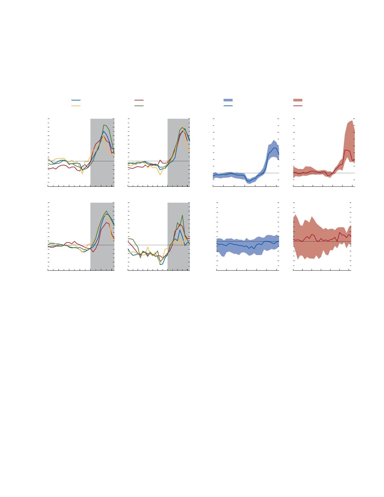
CHAPTER 2 Managing Expectations: Inflation and Monetary Policy

Figure 2.2. Next-12-Months Mean Inflation Expectations by

Figure 2.3. Cross-Economy Distribution of Mean Inflation

Economic Agent

Expectations over Time

( z-score, standard deviations from the mean)

(Percentage point deviation from target)

Economic agents agree on the broad dynamics of near-term inflation expectations.

Near-term inflation expectations shot up rapidly from 2022 but are now reverting,

The sharp increases in 2022 were unusual compared to the experience of the last

while long-term inflation expectations have moved only marginally, but in a

20 years.

narrowing range.

Professional forecasters

Households

AE interquartile range

EME interquartile range

Financial markets

Firms

AE median

EME median

1. United States

2. Euro Area

1. AEs: Next-12-Months

2. EMEs: Next-12-Months

-1

-2

-3

–2

-2

2017

2017 18

3. United Kingdom

4. Brazil

0.8

3. AEs: Five-year-ahead

4. EMEs: Five-year-ahead

0.8

0.6

0.4

0.2

0.0

–0.2

-0.2

-1

-2

–0.4

-0.4

-3

–0.6

-0.6

2017

2017 18

Sources: Consensus Economics; European Commission; Haver Analytics; NL

Sources: Central bank websites; Consensus Economics; Haver Analytics; and IMF

Analytics; S&P Capital IQ; and IMF staff calculations.

staff calculations.

Note: The figure shows z-scores (variable minus its mean, all divided by its

Note: Mean inflation expectations in the figure are from professional forecasters.

standard deviation) calculated over the period 2004:Q1 to 2023:Q2 at quarterly

Economies are included in the sample based on data availability. See Online Annex

frequency. Shaded areas in each panel highlight the period from 2021 onward,

2.1 for details. AEs = advanced economies; EMEs = emerging market economies.

when realized inflation began notably rising.

Near-Term Inflation Expectations above Targets,

fluctuating risk premium is challenging (Chapter 1 of

Long-Term Contained

April 2023 Global Financial Stability Report). Firms’

near-term inflation expectations tend to mark the

When a larger set of economies is examined, a

upper bound of the cross-agents expectations range

consistent picture emerges: near-term inflation expec-

during the recent inflation surge. Professional forecast-

tations in deviation from central banks’ targets have

ers’ expectations convey more signal but may suffer

risen, whereas deviations of long-term expectations

from herding and strategic behavior (Reis 2023).

have been broadly stable (Figure 2.3).⁹

Typically, professional forecasters’ expectations fall

For advanced economies, the period prior to the

somewhere between the more volatile, yet continu-

start of the COVID-19 pandemic in the first quar-

ously available, market-implied and noisier household

ter of 2020 was marked by a mild undershooting of

expectations. Tey also have the advantage of the

inflation expectations relative to target in both the near

broadest coverage among expectations measures across

economies, time, and forecast horizon. As such, the

⁹Central bank inflation targets are either explicit or implicit; see

analyses of the chapter mostly use the expectations of

Online Annex 2.1 for further details on data sources. All online

professional forecasters.

annexes are available at www.imf.org/en/Publications/WEO.

International Monetary Fund | October 2023

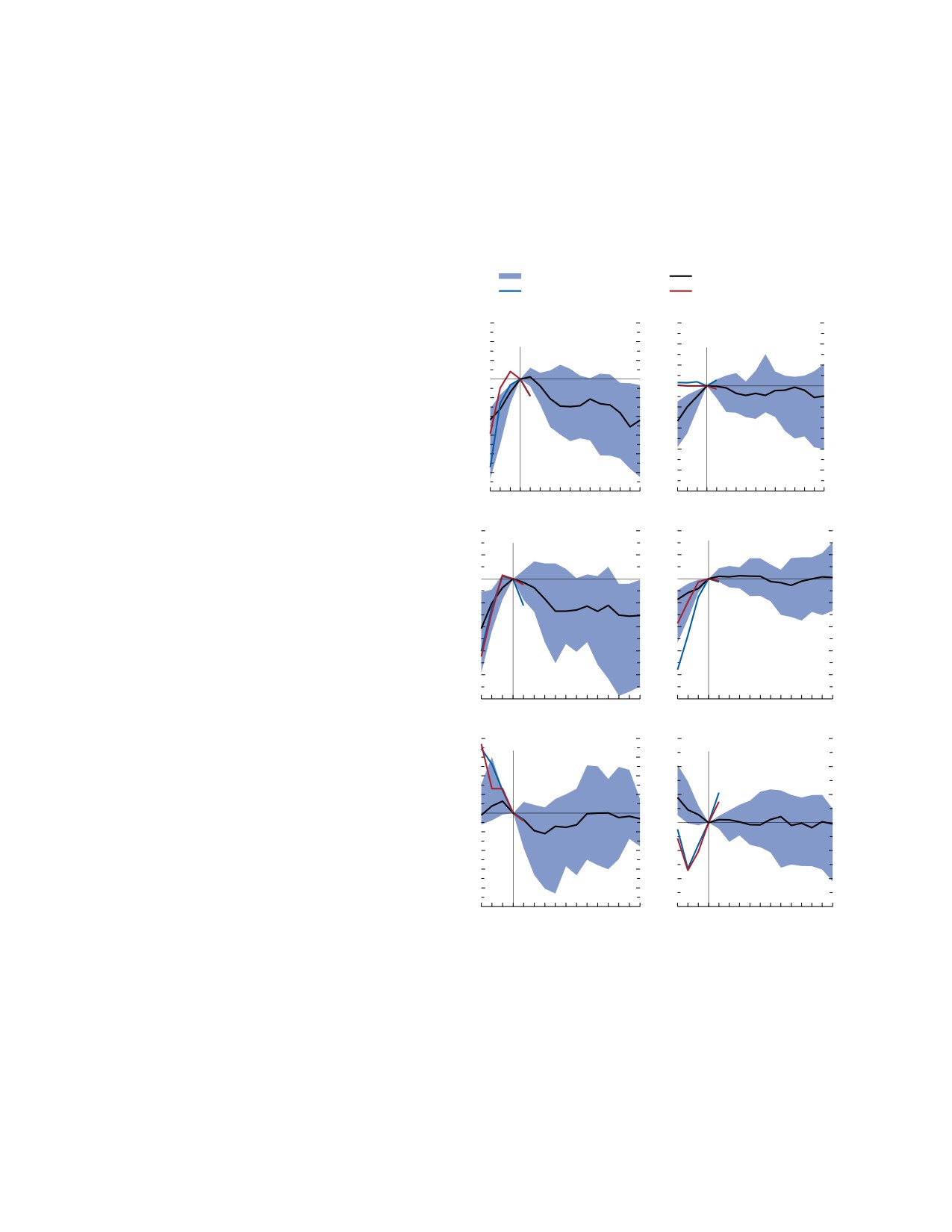
WORLD ECONOMIC OUTLOOK: Navigating Global Divergences

and long terms (Figure 2.3, panels 1 and 3). Near-term

Figure 2.4. Historical Episodes with Persistently Rising

expectations rose markedly after 2021. If anything,

Near- and Long-Term Inflation Expectations

(Percentage points relative to level at end of episode)

long-term expectations in advanced economies have

moved closer to inflation targets since the pandemic.

After past episodes in which inflation expectations rose persistently for a year or

For emerging market economies, the distribution

more, it took about three years on average for inflation and near-term expectations

to come back down to pre-episode levels. Compared with those in these historical

of near-term inflation expectations is somewhat wider

episodes, recent long-term inflation expectations have been unusually stable and

and skewed to the upside, indicating greater variation

real policy rate paths sharper across economy groups.

in inflation experiences, particularly in recent quarters

Interquartile range

Median

(Figure 2.3, panel 2). Median long-term inflation

Median, AEs, 2022:Q4 = 0

Median, EMEs, 2022:Q4 = 0

expectations have moved upward by a modest 10

basis points (Figure 2.3, panel 4). Te interquartile

1.5

1. Near-Term Inflations

2. Long-Term Inflations

0.6

Expectations

range for long-term expectations has narrowed and

1.0

0.4

shifted up somewhat. Overall, though, the patterns

0.5

0.2

suggest that long-term inflation expectations have

0.0

-0.5

remained stable.

-0.2

-1.0

For both advanced and emerging market economies,

-0.4

-1.5

multiple metrics of inflation expectations anchoring—

-0.6

-2.0

related to the average absolute deviations from target,

-2.5

-0.8

variability of expectations over time, and disagreement

-3.0

-1.0

about expectations across individuals—suggest that

-3

long-term inflation expectations have stayed anchored

3. CPI Inflation

4. CPI Core Inflation

despite recent rises in inflation (see Online Annex 2.2).

Although reassuring, this anchoring of long-term

expectations should not be taken for granted—it likely

reflects in part the active response of policymakers to

-1

dampen price pressures.

-2

-3

-4

History Suggests It Can Take Time for Inflation and

Near-Term Expectations to Come Down

-5

-3

Long-term inflation expectations have remained

5. Real Growth

6. Real Policy Rate

stable, but how unusual are the current paths of other

major macroeconomic variables? To put it into histori-

cal context, the chapter compares the recent experience

with that observed after historical episodes in which

near- and long-term inflation expectations were rising

-1

for at least a year (Figure 2.4).

-2

-1

Current paths for actual inflation are so far in line

-3

-2

with historical medians, whereas near-term inflation

-4

expectations displayed a sharper increase and a faster

-5

-3

decline compared with those in previous episodes.

After inflation expectations persistently rose over a

Sources: Consensus Economics; and IMF staff calculations.

Note: Horizontal axes show quarters after the end of the historical episode. All

year, economies subsequently tended to see a gradual

rates are expressed in annual terms. Near-term inflation expectations (panel 1) are

but slow decline in headline inflation and near-term

expected inflation rates over the subsequent year on a rolling basis. Long-term

inflation expectations (panel 2) are expected inflation rates in five years’ time. Real

inflation expectations. Both typically take about three

policy rates are interest rates based on expected inflation. Inclusion as a historical

years to revert to their pre-episode levels, although

episode requires four quarters in which both near- and long-term inflation

core inflation remained stickier. However, there is a

expectations are rising. The sample spans 1989:Q4 to 2023:Q1, with exact time

coverage varying by economy. A total of 32 historical episodes are identified, with

large variability across experiences, as observed in the

16 from AEs and 16 from EMEs. See Online Annex 2.3 for further details.

interquartile ranges.

AEs = advanced economies; CPI = consumer price index; EMEs = emerging

market economies.

International Monetary Fund | October 2023

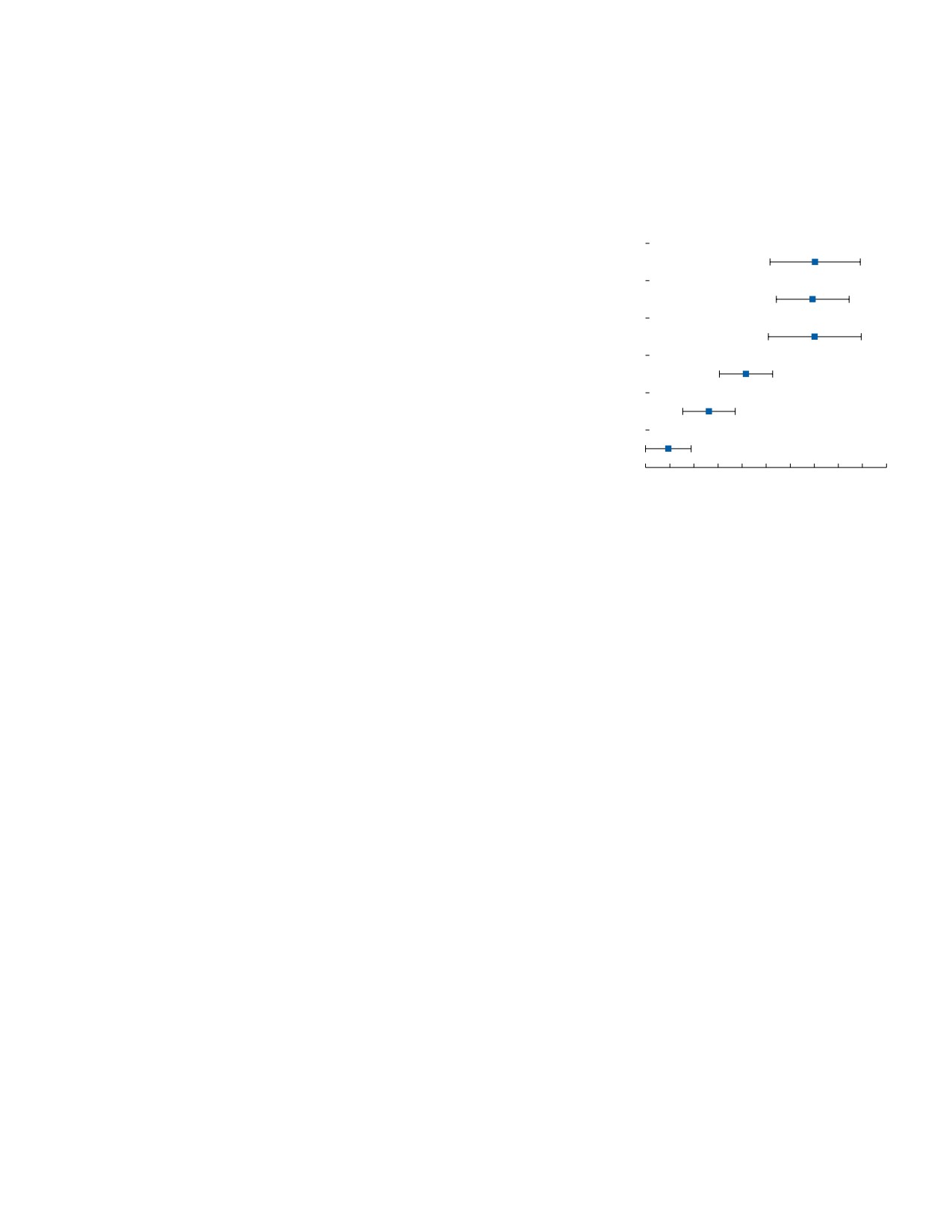
CHAPTER 2 Managing Expectations: Inflation and Monetary Policy

In contrast, recent paths for real policy rates and

Figure 2.5. Estimated Effects of Alternative Inflation

long-term inflation expectations appear different than

Expectations Measures on Current Inflation

(Standardized regression coefficients)

the median paths in past episodes. On the one hand,

real policy rates in 2022 were well below those in

Near-term measures of inflation expectations can better predict current inflation

the comparative paths of earlier episodes, partly on

than longer-term measures. Expectations of firms, financial markets, and

professional forecasters show similar performances.

account of the sharp and large rise in inflation. On the

other hand, real rates are now well above the historical

median, with the difference reflecting rapid monetary

Professional forecasters NT

tightening and the latest falls in headline inflation.

Unlike those in earlier episodes, long-term inflation

Financial markets NT

expectations have been unusually stable coming into

Firms NT

the recent high inflation regime. Tis is consistent

with and supports the chapter’s findings on the recent

Households NT

stability and (so far) solid anchoring of long-term

expectations.

Financial markets LT

Professional forecasters LT

The Role of Expectations in Inflation Dynamics

0.0

0.1

0.2

0.3

0.4

0.5

0.6

0.7

0.8

0.9

1.0

To provide a better understanding of the role of

expectations in inflation dynamics, this section con-

Source: IMF staff calculations.

siders a hybrid price Phillips curve framework that

Note: The figure shows standardized coefficients from linear regressions

estimated by pooled time series for the euro area, United Kingdom, and United

relates current inflation to a set of drivers, including

States using quarterly data from 1991:Q2 through 2023:Q1. The dependent

inflation expectations, lagged inflation, and the out-

variable is quarterly headline inflation, seasonally adjusted at an annualized rate.

put gap.¹⁰ Te section first assesses the explanatory

See Online Annex 2.4 for details on the regression specification and additional

control variables. Horizontal lines show 90 percent confidence intervals with

power of different agents’ expectations for inflation

heteroskedasticity-robust standard errors. LT = long-term (five-year-ahead; for

and the relative importance of near- versus long-term

financial markets is next-five-years) inflation expectations; NT = near-term

(next-12-months) inflation expectations.

expectations. Second, an instrumental variables

approach is used to identify the causal impact of

inflation expectations on inflation. Tird, using the

Near-Term Expectations Matter Most for Inflation

causal estimates, the section shows the contributions

When considered one by one, alternative measures of

of different drivers to recent inflation dynamics for

inflation expectations (by agents or horizons) show differ-

average advanced and emerging market economies.

ent abilities to explain inflation when the hybrid Phillips

Finally, the section explores whether the effect of

curve model is used (Figure 2.5). Te coefficient esti-

expectations on inflation changes with the prevailing

mates represent the change in inflation associated with a

level of inflation.¹¹

one standard deviation increase in the indicated measure

of expectations.¹² Te first finding is that long-term

inflation expectations have lower predictive power than

near-term measures. Both financial-market-based and

¹⁰See Chapter 3 of the October 2018 World Economic Outlook

professional forecasters’ five-year-ahead inflation expec-

(WEO), Chapter 2 of the October 2021 WEO, and Chapter 2

tations have smaller standardized coefficients than other

of the October 2022 WEO for recent analyses looking at

measures (Figure 2.5, bottom two sets of boxes and whis-

cross-economy estimates of Phillips curves (for prices and

wages). Dao and others (2023) use a similar approach to analyze

kers). Tese results are consistent with those of recent

inflation developments in the United States and the euro area.

See Online Annex 2.4 for further details on the estimation

and analysis.

¹²Te coefficients are standardized to account for the volatility of

¹¹Other potential important dimensions in modeling the Phillips

different measures and to allow a comparison of inflation forecasts

curve relationship, such as time-varying coefficients, nonlinearities,

with the new index of firms’ inflation expectations, which is based

structural breaks, and the influence of higher-order moments of

on a different scale. Because of lack of data availability, this compar-

measured expectations, as well as alternative measures of slack, are

ison can be undertaken for the United Kingdom, the United States,

left for future work.

and the euro area.

International Monetary Fund | October 2023

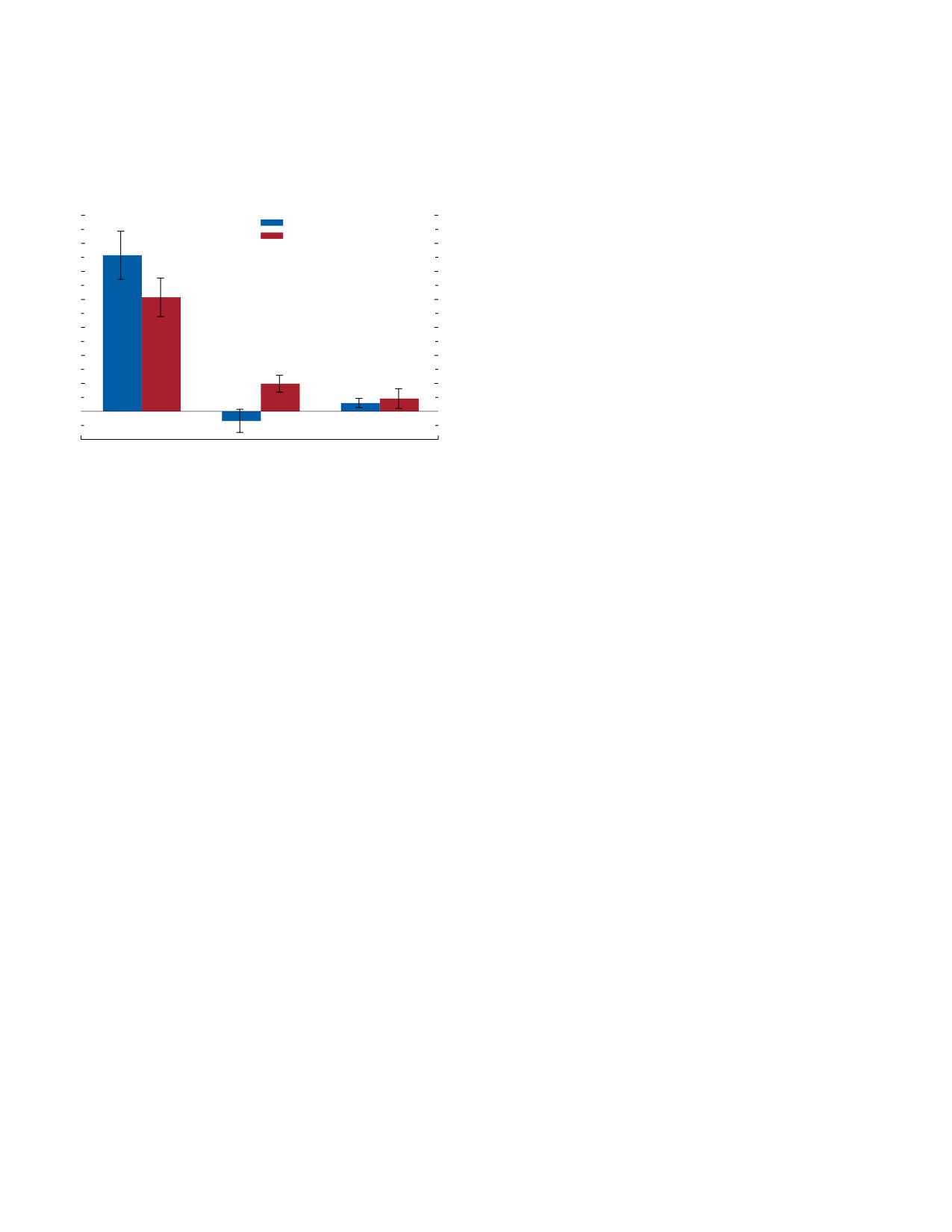
WORLD ECONOMIC OUTLOOK: Navigating Global Divergences

Figure 2.6. Key Coefficients of the Hybrid Phillips Curve

0.8 percentage point. Lagged inflation has little explan-

(Regression coefficients)

atory power in advanced economies (slightly negative

but not different from zero with statistical significance),

Near-term inflation expectations play a larger role in explaining current inflation in

advanced economies than in emerging market economies.

whereas in emerging market economies, the carryover

from the previous quarter’s inflation (about 0.2 percent-

1.4

Advanced economies

age point) is statistically significant.¹⁴ Finally, the output

Emerging market economies

1.2

gap has a statistically significant relationship with cur-

rent inflation for both economy groups but is somewhat

1.0

larger for the group of emerging market economies.

0.8

0.6

Expectations’ Role for Inflation May Be Smaller Than

0.4

Simple Statistical Associations Suggest

0.2

Te previous results document statistical associa-

tions between current inflation and near-term inflation

0.0

expectations—they do not account for the possibility

-0.2

that current inflation could drive expectations of future

Near-term expectations

Lagged inflation

Output gap

inflation or that omitted factors could be driving both.

Source: IMF staff calculations.

To address these shortcomings and estimate the causal

Note: The figure shows coefficients from linear regressions estimated by pooled

effect of expectations on inflation (the expectations

time series using quarterly data from 1991:Q2 through 2023:Q1. The dependent

variable is quarterly headline inflation, seasonally adjusted at an annualized rate.

channel), an instrumental variables strategy based on

See Online Annex 2.4 for details on the regression specification and additional

lags of near-term inflation expectations and the output

control variables. Whiskers show the 90 percent confidence intervals with

Driscoll-Kraay standard errors.

gap is used to reestimate the hybrid Phillips curve. Te

strategy leverages the facts that these variables display

serial correlation over time (current values are strongly

work that finds a small role for long-term expectations

related to their past values) and that lags of these vari-

on current inflation (Werning 2022; Hajdini 2023). Sec-

ables do not directly affect current inflation under the

ond, there is remarkable consistency across professional

hybrid Phillips curve specification.¹⁵

forecasters’, financial markets’, and firms’ near-term infla-

tion expectations (Figure 2.5, top three boxes and whis-

¹⁴Chapter 3 of the October 2016 World Economic Outlook (WEO)

kers). Tese results imply that a one-standard-deviation

and Chapter 2 of the October 2016 and October 2021 WEO,

increase in expectations is associated with a 0.7 standard

respectively, as well as Kamber, Mohanty, and Morley (2020), also

find higher coefficients for lagged inflation in hybrid Phillips curves

deviation increase in current inflation.¹³ Finally, the

in emerging market economies compared with those in advanced

coefficient for households’ near-term expectations falls

economies. Forbes, Gagnon, and Collins (2021) demonstrate that

somewhere between those for near- and long-term expec-

the coefficients on lagged inflation decrease when panel estimates

tations of other agents.

include only advanced economies. Tese studies do not explore

potential causes, but the higher prevalence of price indexation in

In light of these findings and crucially because of

many emerging market economies may account for these findings

broader economy and time coverage, the baseline spec-

(Céspedes and others 2005; Frankel 2010; Kganyago 2023). In

ification of the hybrid Phillips curve is estimated using

addition, weaker monetary policy frameworks, on average, could also

contribute to the smaller relative role of expectations. It might also

near-term inflation expectations from professional fore-

be rational for adaptive learners to rely more on past inflation when

casters (Figure 2.6). Te estimated relationship suggests

indexation is more prevalent and the credibility of policymaking

that a 1 percentage point rise in near-term expectations

institutions is lower. Improvements in monetary policy frameworks

and communications in emerging market economies over the past

is associated with a 1.1 percentage point rise in cur-

15 years (see Box 2.2) suggest that lagged inflation could play a

rent inflation among advanced economies, whereas

reduced role in these economies’ inflation dynamics going forward.

for emerging market economies, the rise is about

Finally, emerging market economies might suffer from larger mea-

surement error on inflation expectations, which would lead to an

attenuation bias and a relatively more important estimated role for

¹³Coefficients for inflation expectations unadjusted for volatility

lagged inflation.

range from 1.1 to 1.4. Te estimated coefficients for long-term

¹⁵See Online Annex 2.4 for further details on the model specifica-

expectations are lower than those for near-term expectations. Exclud-

tion, instrumental variables strategy, its performance and key results,

ing the post-2019 period results in lower estimated coefficients, but

and robustness checks. Te instrumental variables estimates are stable

similar patterns.

across time periods.

International Monetary Fund | October 2023

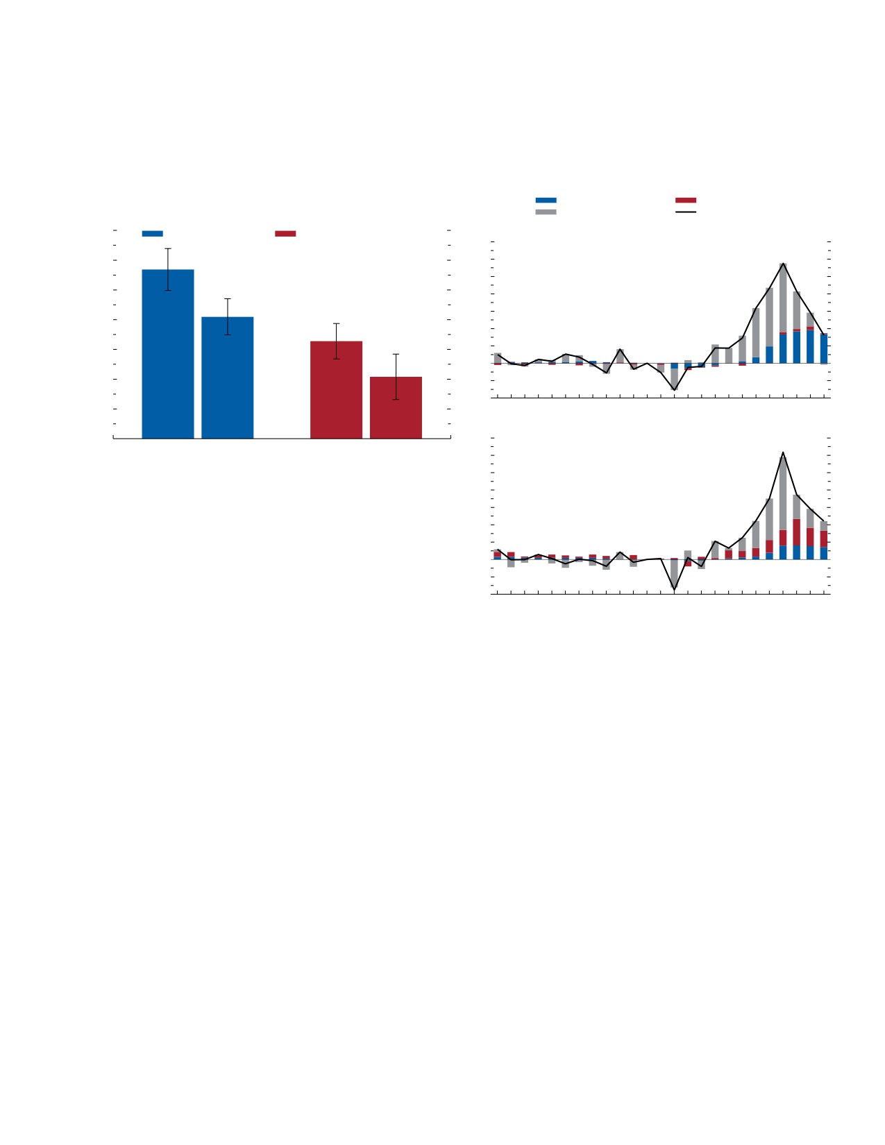
CHAPTER 2 Managing Expectations: Inflation and Monetary Policy

Figure 2.7. Associational versus Causal Estimated Effects of

Figure 2.8. Contributors to Recent Inflation Dynamics

Inflation Expectations on Current Inflation

(Percentage point deviation from 2019:Q4)

(Regression coefficients)

A decomposition of the recent dynamics of headline inflation reveals the growing

importance of near-term inflation expectations.

Accounting for the influence of current inflation on expectations of future inflation

in the Phillips curve reduces the estimated effects of inflation expectations on

current inflation by about 30 percent across economy groups.

Near-term expectations

Lagged inflation

All other factors

Headline inflation

1.4

Advanced economies

Emerging market economies

1. Advanced Economies

1.2

1.0

0.8

0.6

0.4

-2

-4

0.2

2017

0.0

2. Emerging Market Economies

Associational

Causal

Associational

Causal

Source: IMF staff calculations.

Note: The figure shows coefficients from linear regressions estimated by pooled

time series using quarterly data from 1991:Q2 through 2023:Q1. Whiskers show

the 90 percent confidence interval around the estimated coefficient. The

dependent variable is quarterly headline inflation, seasonally adjusted at an

annualized rate. Associational estimates are computed by ordinary least squares,

while causal estimates are computed using an instrumental variables approach.

Models include economy and time fixed effects along with additional control

-2

variables. See Online Annex 2.4 for further details on the specification and

instrumental variables strategy.

-4

2017

Source: IMF staff calculations.

Te causal estimates of the effects of near-term

Note: Bars in the figure show the contributions to average headline inflation by

expectations on current inflation are about 30 per-

economy group relative to the contributions observed in 2019:Q4. Contributions

are calculated using coefficients estimated by instrumental variables pooled time

cent lower in magnitude than the associational

series with quarterly data over 1991:Q2-2023:Q1. The black lines in each panel

estimates (Figure 2.7). Tis implies that some

show the average seasonally adjusted annualized quarter-on-quarter headline

consumer price index inflation observed relative to 2019:Q4. The “All other

of the observed variation in near-term inflation

factors” category includes the contributions from time fixed effects (common

expectations reflects reverse causation (that is,

global factors), all other explanatory variables, and the regression residual. See

Online Annex 2.4 for details on the specification and estimation.

higher current inflation drives up expectations of

future inflation) or omitted factors that affect both

current inflation and expectations. By removing

Expectations Explain an Increasing Share of Recent

these biases, the instrumental variables estimates

Inflation Dynamics

provide a more accurate assessment of the expecta-

tions channel. For the average advanced economy,

Te contribution to recent inflation dynamics of the

inflation would rise by about 0.8 percentage point

expectations channel can be calculated using the causal

for a 1 percentage point rise in near-term expec-

estimates of the hybrid Phillips curve (Figure 2.8).

tations. Te pass-through estimate for the average

For the average advanced economy, factors other

emerging market economy is about 0.4 percentage

than expectations and lagged inflation initially drove

point. Te difference in magnitudes, combined with

most of the increase in inflation that took place over

differences in the relationship of current inflation to

2021-22 (Figure 2.8, panel 1). Tese include common

past inflation, suggests that expectations formation

global factors, such as the economic disruptions caused

in emerging market economies on average tends to

by the COVID-19 shock, large swings in commod-

be more backward looking than what is observed in

ity prices, and global supply chain issues, as well as

advanced economies.

the economy-specific effects of energy prices and the

International Monetary Fund | October 2023

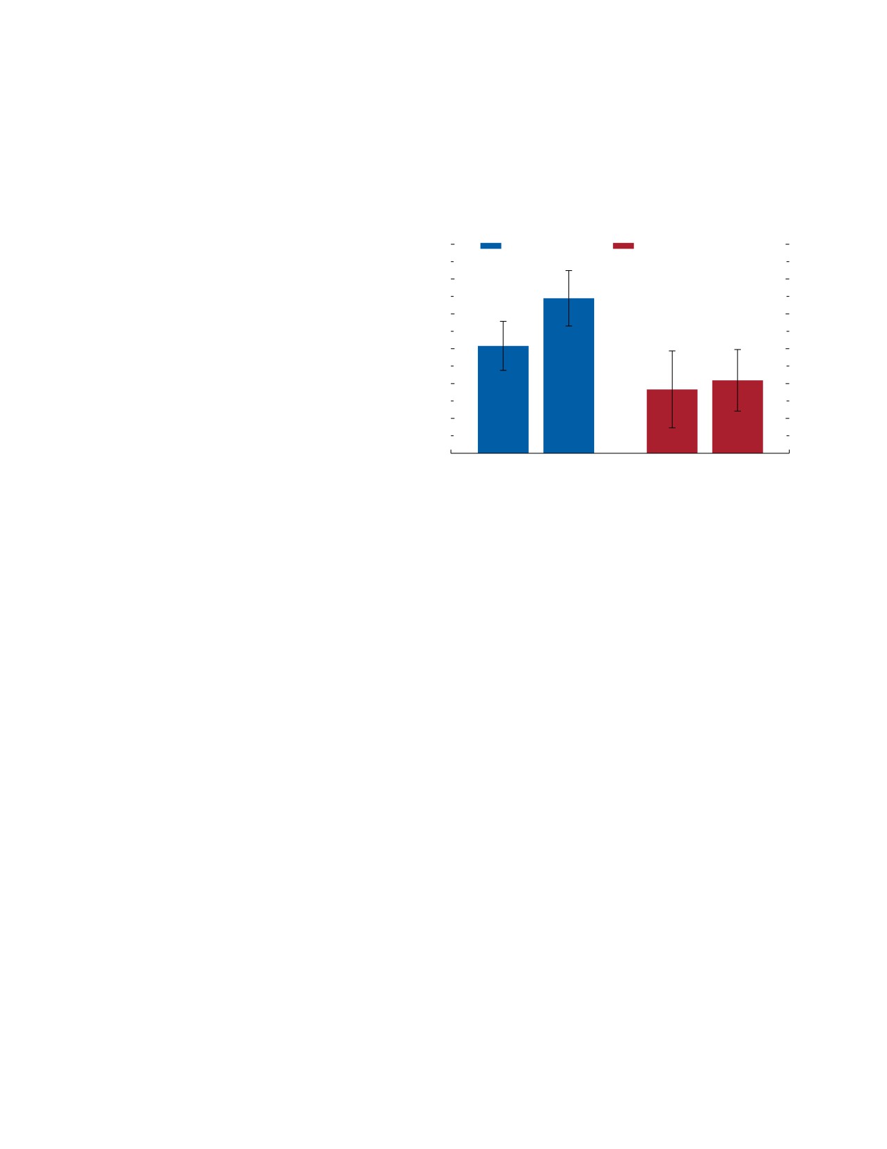
WORLD ECONOMIC OUTLOOK: Navigating Global Divergences

output gap (which may in turn reflect domestic aggre-

Figure 2.9. State-Dependent Pass-Through from

gate demand measures). Even so, Figure 2.8 reveals a

Expectations to Inflation

(Regression coefficients)

large and growing role for near-term inflation expec-

tations in explaining inflation dynamics in the most

The pass-through (or effect) from inflation expectations to current inflation is

recent quarters.¹⁶ In contrast, lagged inflation had a

higher when the prevailing level of inflation is higher across economy groups. The

difference in pass-through by prevailing level of inflation is larger for advanced

small role.

economies.

Turning to the average emerging market economy,

once again factors other than expectations and lagged

1.2

Advanced economies

Emerging market economies

inflation were responsible for the peak in inflation in

2022 (Figure 2.8, panel 2). On average, expectations

1.0

have played a significant but smaller role in accounting

0.8

for headline inflation than among advanced econo-

mies. On the other hand, lagged inflation explained

0.6

almost half of the average rise in inflation since the

first quarter of 2020.

0.4

0.2

Higher Inflation Environment, Higher Pass-Through

from Expectations

0.0

Low

High

Low

High

Te final exercise in the section consists of esti-

mating whether the pass-through from inflation

Source: IMF staff calculations.

expectations to current inflation varies by the level

Note: Bars in the figure show the average estimated coefficients from regressions

of headline inflation on inflation expectations by economy group, interacted with

of inflation: Are there signs of a nonlinearity or state

an indicator for whether lagged headline inflation was above an economy’s

dependence in the effect of expectations on inflation?

median inflation level over the sample period. Estimation is via instrumental

variables using quarterly data over 1991:Q2-2023:Q1. See Online Annex 2.4 for

In both advanced and emerging market economies,

further details on the regression specification and estimation. The whiskers show

the estimated pass-through is higher when inflation is

the 90 percent confidence interval using heteroskedasticity-robust standard errors.

elevated (above its economy-specific sample median;

Figure 2.9). Te difference is particularly large, with

the coefficient increasing from 0.6 when inflation is

interact with monetary policy actions, affecting

low (below its economy-specific sample median) to

the dynamics of inflation, expectations, and eco-

0.9 when inflation is high and statistically significant

nomic activity.

for advanced economies. Tese results imply that the

Te analysis extends the standard dynamic sto-

expectations channel may be even more important in

chastic general equilibrium model with expectational

accounting for inflation dynamics at present, while

learning by Alvarez and Dizioli (2023). Te model

inflation remains high.

includes price and wage Phillips curves (relating

price and wage inflation to expectations, the gap

between real wages and productivity, and economic

Expectations Formation and Monetary

slack), an IS curve (relating output to the nomi-

Policymaking

nal interest rate and inflation expectations), and

Tis section explores the question of how infla-

a monetary policy reaction function.¹⁷ Two new

tion expectations affect monetary policy effectiveness

features are incorporated into the model. First,

and how different policies can affect expectations.

heterogenous agents or a mix of backward- and

It uses a semistructural model to illustrate how the

forward-looking learners with different information

expectations formation processes in an economy

sets are added. Backward-looking learners form

their expectations based on their recent experience,

whereas forward-looking learners form their expecta-

¹⁶Other factors have remained relevant in recent quarters despite

tions rationally based on full information about the

a net contribution approaching zero, as shown by the gray bars in

Figure 2.8, panel 1. Tis is because the pass-through from lower

energy prices has been offset by other factors, mainly captured by

¹⁷See Online Annex 2.5 for more details about the model, its

quarterly fixed effects.

structure, and its estimation.

International Monetary Fund | October 2023

CHAPTER 2 Managing Expectations: Inflation and Monetary Policy

economy, including the share of backward-looking

panels 1-4). Moreover, with heterogenous agents,

learners. Tis means that forward-looking learners

monetary policy has less power initially to influence

will behave more like backward-looking learners

inflation (Figure 2.10, panels 5-8). Te main reason

as the share of backward-looking learners rises in

is that backward-looking learners do not consider

the economy.¹⁸ Second, as inspired by Blanchard and

the impact of monetary policy on future marginal

Bernanke (2023), near-term expectations are influ-

costs, unlike forward-looking learners. Without this

enced by long-term expectations and vice versa. Te

forward-looking component, monetary policy can

main additional assumption is that long-term expec-

influence expectations only through its direct effects

tations have an impact on inflation only through

on the output gap.

their effect on near-term expectations. An alternative

model allowing only forward-looking learners is

Higher Sacrifice Ratio with More Backward-Looking

also considered for comparison. Te two models—

Learners or Higher Inflation

heterogenous expectations and forward-looking

learners or rational expectations only—are esti-

Te combination of more prolonged inflationary

mated for two representative economies (advanced

episodes following a cost-push shock and less pow-

and emerging market) to help capture the struc-

erful monetary policy implies that achieving a given

tural differences between the two economy groups.

level of inflation reduction over a given period will

With heterogenous agents, the estimated shares of

be more costly in terms of output forgone. Tis will

backward-looking learners are about 20 percent for

be reflected in the level of the sacrifice ratio, defined

the advanced economy and about 30 percent for the

here as the percentage of output forgone to achieve

emerging market economy, with the remainder being

a 1 percentage point faster reduction in the inflation

forward-looking learners.

rate over a three-year period (Figure 2.11).¹⁹ First,

the sacrifice ratio is larger in the heterogeneous

agents’ model than in the rational expectations

More Backward-Looking Learners Prolong Inflation and

model with only forward-looking learners (regardless

Weaken Monetary Policy Transmission

of the economy group). Te main reason for this

Te propagation of shocks to the economy depends

increased sacrifice ratio is the weaker inflation expec-

upon how expectations are formed. Following an

tations channel for monetary policy when there are

identical cost-push shock (for example, a surprise

more backward-looking learners in the economy.

rise in energy and commodity prices, an unantici-

Second, the sacrifice ratio also tends to be higher

pated supply chain disruption raising input costs,

for an emerging market than an advanced economy,

or other supply-side shocks), inflation is persistently

as the former is estimated to have a higher share

higher when there are heterogenous agents in the

of backward-looking learners. Tird, when there

economy, as compared with an economy that has

are heterogenous agents, the economy’s dynamics

only forward-looking learners. With a share of

become state dependent. In a high-inflation environ-

backward-looking learners in the economy, inflation

ment, backward-looking learners behave as though

expectations respond more to a cost-push shock and

inflation will be permanently higher, entailing

are stickier. Backward-looking learners assume that

a slight endogenous inflation de-anchoring and

higher current inflation means that future inflation

making monetary policy’s job harder (Figure 2.11,

will be persistently higher. Tis prolongs the price

rightmost bars).²⁰

pressures compared with those in the economy

with forward-looking learners who know that the

cost-push shock is transitory and do not change

¹⁹Tetlow (2022) reports a wide range of sacrifice ratio estimates

their inflation expectations much (Figure 2.10,

for advanced economies, with a mode of seven (similar to that

presented here) across 40 different models and slightly different

definitions. Tat said, the chapter’s focus is on the qualitative com-

¹⁸Other expectations formation processes are possible (for exam-

parison across cases.

ple, completely anchored, unresponsive inflation expectations). Te

²⁰To get closer to current conditions, a high-inflation environment

chapter does not aim to be exhaustive. It illustrates instead how a

is simulated by running the model for eight periods, with inflation

plausible mix of two highly relevant kinds of processes may affect

2 percentage points above target, to establish the initial conditions

developments.

for the scenario.

International Monetary Fund | October 2023

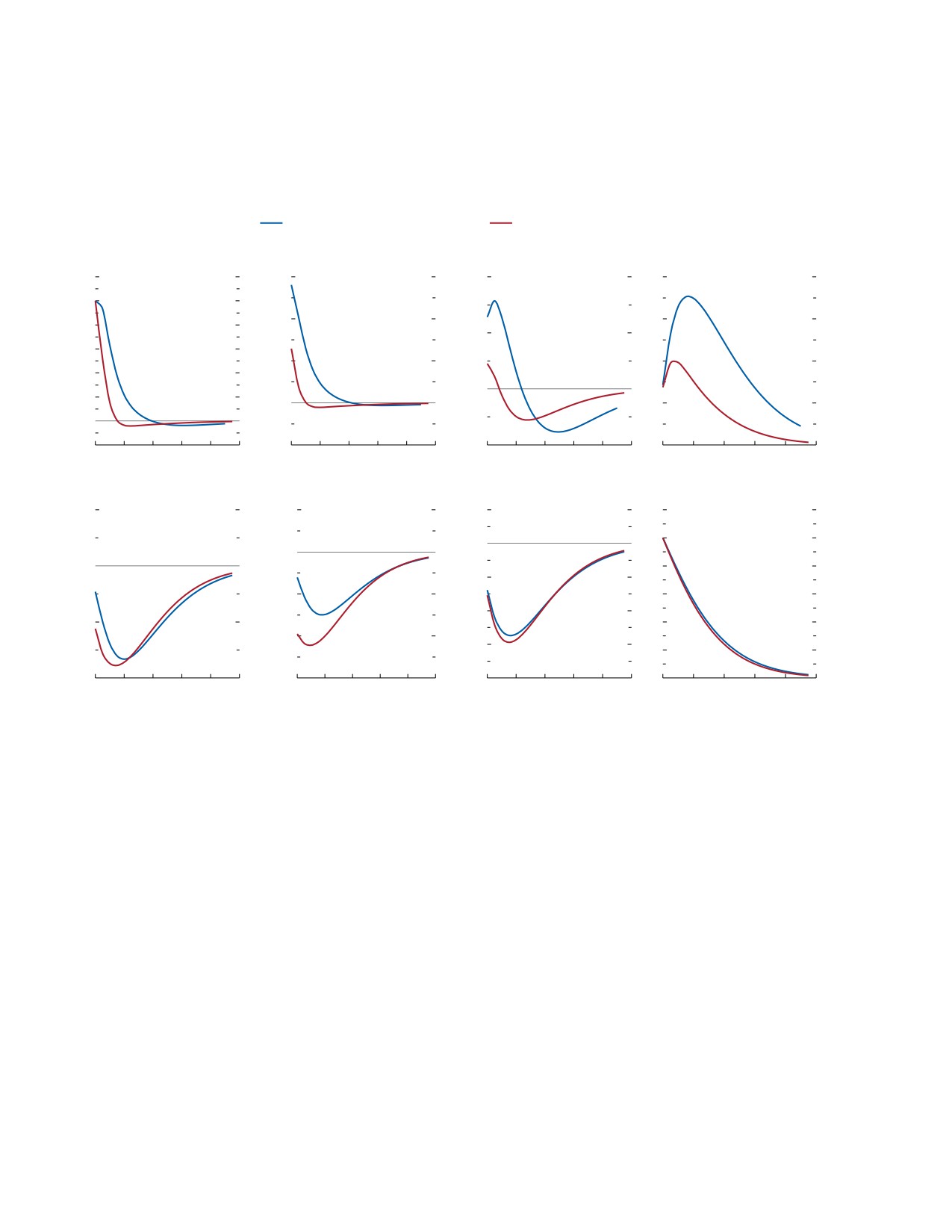
WORLD ECONOMIC OUTLOOK: Navigating Global Divergences

Figure 2.10. Macroeconomic Responses to Shocks Conditional on Agents’ Expectations Formation

(Percentage points)

Following a cost-push shock, inflation expectations are more sensitive when the economy has a mix of forward- and backward-looking learners (heterogenous

expectations) than when it has only forward-looking learners (rational expectations). Inflation is also more persistent. Monetary policy is less effective, as

backward-looking learners do not take account of the effects of interest rate rises on future marginal costs.

Heterogeneous expectations model

Rational expectations model

Cost-Push Shock

1.2

1. Inflation

0.3

2. Near-Term Inflation

0.2

3. Output Gap

4. Policy Interest Rate

0.4

Expectations

1.0

0.2

0.3

0.8

0.1

0.6

0.1

0.2

0.4

0.0

0.2

0.0

0.1

0.0

–0.2

-0.1

0.0

Monetary Policy Shock

0.1

5. Inflation

0.02

6. Near-Term Inflation

0.1

7. Output Gap

8. Policy Interest Rate

1.2

Expectations

1.0

0.0

0.00

0.0

0.8

-0.1

-0.02

0.6

-0.2

-0.1

0.4

-0.04

-0.3

0.2

–0.2

–0.06

-0.4

0.0

Source: IMF staff calculations.

Note: Numbers on the horizontal axes in the panels represent quarters after the shock at time 0. Panels 1-4 show the impulse responses to a cost-push shock that

increases inflation by 1 percentage point. Note that the output gap increases after this shock, because potential output falls by more than real GDP. Panels 5-8 show

the impulse responses to a temporary monetary policy shock that increases the policy rate by 100 basis points. Note that the monetary policy shock’s impact on

inflation peaks after five quarters in the heterogenous-expectations model and after three quarters in the rational-expectations model.

Monetary Policy Framework and Communications

Recent studies suggest that improvements in mone-

Improvements Ease Disinflation

tary policy frameworks—encompassing central banks’

Te estimated model offers a laboratory for consid-

independence and transparency and their communi-

ering how alternative policy interventions help hasten

cations strategies—can increase agents’ attention to

a decline in inflation. Te first intervention examined

and understanding of monetary policy actions, helping

is one that would lead to an increase in the share of

to make inflation expectations more forward looking

forward-looking learners in the economy.²¹ How might

(Coibion and others 2020; Carotta, Mello, and Ponce

such a shift be achieved?

2023). Brazil’s recent decision to adopt a continuous

(rather than calendar year) 3 percent inflation rate target

²¹Several studies over the past several years indicate that most individ-

from 2025 onward is a concrete example of an improve-

uals do not understand the central bank’s role in the economy and how

policy rate changes affect the economy, suggesting that their expectations

ment in operational effectiveness and communications

may be distorted. See, among others, Coibion, Gorodnichenko, and

strategy, helping to reduce uncertainty and enhance

Weber (2022), ECB (2021), Kumar and others (2015), and van der

monetary policy effectiveness. Additional examples of

Cruijsen, Jansen, and de Haan (2015). Andre and others (2022) find that

improvements in communications strategies include

over a sample of 6,500 US households, households on average believe

that a rise in a central bank’s policy interest rate would increase inflation.

actions since 2020 by the central banks of Pakistan

International Monetary Fund | October 2023

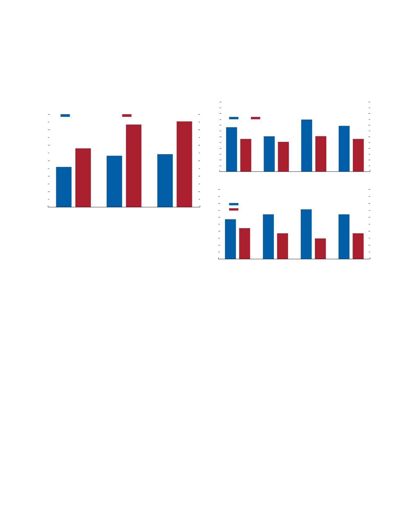
CHAPTER 2 Managing Expectations: Inflation and Monetary Policy

Figure 2.11. Sacrifice Ratios under Alternative Expectations

Figure 2.12. Soundness of Monetary Policy Frameworks and

Processes

Forecast Rationality Tests across Economies

(Percent of output forgone to lower inflation by 1 percentage point)

Monetary policy frameworks in advanced economies score higher along multiple

Sacrifice ratios are larger when economies include a mix of forward- and

dimensions, on average, than do those in emerging market and developing

backward-looking learners (heterogenous expectations), as monetary policy is less

economies. Forecast rationality is statistically rejected more often for economies

effective in that case. Emerging market economies tend to have higher shares of

that have lower-quality monetary policy frameworks.

backward-looking learners, pushing up their ratios. Higher prevailing inflation

slightly worsens the ratio, as backward-looking learners raise their expectations.

1.2

1. Qualities of Monetary Policy Frameworks

(Indicator from 0 to 1, higher = more sound)

Advanced economies

Emerging market economies

1.0

AEs

EMDEs

0.8

0.6

0.4

0.2

0.0

IAPOC

POS

COM

2. Percentage of Economies in Which Forecast Rationality Is

Rejected Conditional on Monetary Policy Framework Quality

Lower tier

Upper tier

Rational-expectations

Heterogenous-

model

expectations

model

model with high inflation

Source: IMF staff calculations.

Note: The sacrifice ratios in the figure are calculated under the assumption that

monetary policy is implemented to bring the inflation rate down by 1 percentage

point over three years. See Online Annex 2.5 for further details on the dynamic

stochastic general equilibrium model.

IAPOC

POS

COM

Sources: Unsal, Papageorgiou, and Garbers (2022); and IMF staff calculations.

and Uruguay to announce their preset monetary policy

Note: Panel 1 shows the mean of the indicator by economy group for which data

are available (2007-21). Panel 2 of the figure shows the share of economies

meeting calendar in advance. Additional examples

(among those with expectations from professional forecasters) for which a simple

of improvements in operational effectiveness include

forecast rationality test (Lovell 1986) rejects the hypothesis of rational

expectations. See Online Annex 2.7 for further details. AEs = advanced

decisions since 2019 by the central banks of Chile

economies; EMDEs = emerging market and developing economies; IAPOC =

and Tailand to state their primary policy objective as

Overall Monetary Policy Framework index, which is composed of three pillars:

Independence and Accountability (IA), Policy and Operational Strategy (POS), and

price stability, with clearly defined numerical targets.

Communications (COM).

Trough the lens of the model, the chapter quantifies

the potential effects of such interventions in a stylized,

illustrative manner.

Further bolstering the evidence on the importance of

Moreover, an association exists between the qualities

the soundness of monetary policy frameworks, a nega-

of the monetary policy framework in an economy and

tive association exists between the size of deviations of

the likelihood that a simple forecast rationality test of

near-term inflation expectations (or realized inflation

mean inflation expectations is rejected (Figure 2.12; see

rates) from targets and the quality of monetary policy

also Online Annex 2.5). When monetary policy frame-

frameworks. As monetary policy frameworks improve,

works are weaker (in terms of central bank indepen-

the deviations from target are smaller, implying that

dence, transparency, and communications), the share

inflation comes back to target more quickly, on average

of economies in which forecast rationality of expec-

(see Online Annex 2.7).

tations is rejected tends to be higher, consistent with

Although there has been a notable trend toward

a greater incidence of backward-looking learners.²²

improving frameworks in emerging market and develop-

ing economies (Box 2.2), the quality of monetary policy

frameworks and communications is higher, on average,

²²Te monetary policy framework indicators come from Unsal,

Papageorgiou, and Garbers (2022). See also Box 2.2.

in advanced economies than in emerging market and

International Monetary Fund | October 2023

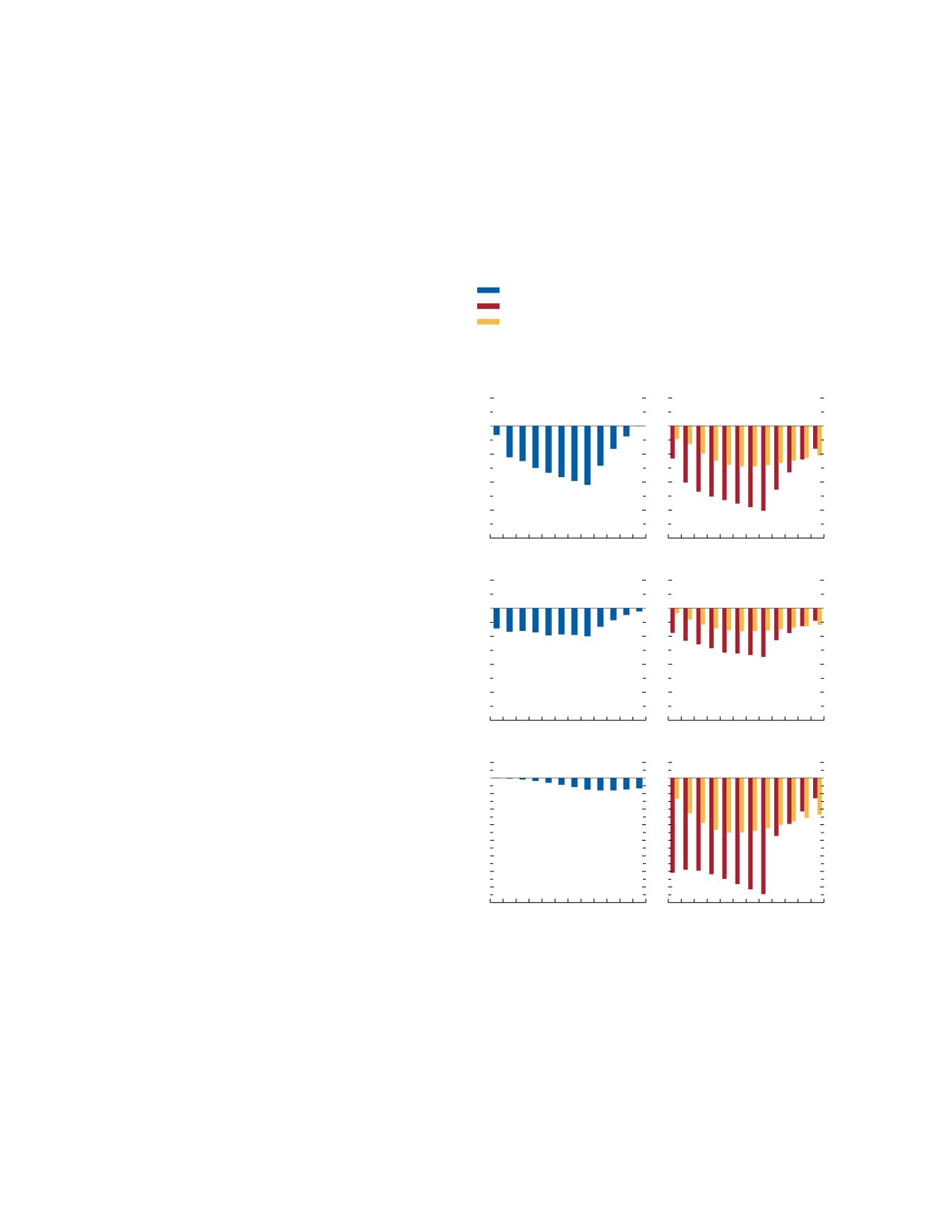
WORLD ECONOMIC OUTLOOK: Navigating Global Divergences

developing economies. As such, the analysis of the

Figure 2.13. Policy Interventions to Hasten the Reduction of

policy intervention considers a decline in the share of

Inflation and Inflation Expectations

(Percentage point, deviation from baseline)

backward-looking learners in the economy equal to

the difference between the share of backward-looking

Improvements in the monetary policy framework and communications strategy

learners in the representative emerging market versus

that boost the share of forward-looking learners in the economy improve the

trade-off between lowering inflation and fostering growth through their effects on

that in the representative advanced economy.²³ With

the expectations channel. Tighter cyclical policies—fiscal consolidation and

a higher share of forward-looking learners, the same

monetary tightening—also lower inflation and inflation expectations, but at a

monetary policy tightening path as under the baseline

higher output cost.

would have stronger effects on inflation expectations

Monetary policy framework and communications strategy improvements

(Figure 2.13, panels 1, 3, and 5). Monetary policy is

Fiscal consolidation

more effective not only because forward-looking learners

Monetary tightening

understand the impacts on future marginal costs, but

Monetary Policy

Tighter Cyclical

also because they know that that there is a lower share

Framework Improvements

Policies

of backward-looking learners in the economy and hence

0.1

1. Inflation

2. Inflation

0.1

become even more forward looking. Tese results are

consistent with findings highlighted in Box 2.1, in

0.0

which US monetary policy is found to be more effective

-0.1

in shaping expectations when firms are more attentive to

monetary policy than the average firm in the sector and

-0.2

therefore are more forward looking. Te faster trans-

-0.3

mission to inflation expectations translates into a lower

-0.4

realized inflation path and importantly a softer landing,

with only small additional output costs.

0.1

3. Inflation Expectations

4. Inflation Expectations

0.1

In contrast, even tighter cyclical policies (either

monetary or fiscal) as additional interventions also help

0.0

dampen inflation and expectations, but come with

–0.1

-0.1

larger output costs (Figure 2.13, panels 2, 4, and 6).

While the two cyclical policy interventions are not

–0.2

-0.2

strictly comparable, they both work in part through

–0.3

-0.3

generating lower aggregate demand initially.²⁴ Over

–0.4

-0.4

time, then, the inflation-lowering effects of tighten-

ing feed into inflation expectations, further lowering

0.1

5. Output Gap

6. Output Gap

0.1

realized inflation.

0.0

Although an improvement in monetary policy

–0.1

-0.1

framework and communications comes with mark-

–0.2

-0.2

edly lower output costs due to its primary impacts

–0.3

-0.3

–0.4

-0.4

on expectations and their formation, difficulties in

–0.5

-0.5

implementing these interventions in a timely and effec-

–0.6

-0.6

tive manner mean that they are not silver bullets and

–0.7

-0.7

–0.8

-0.8

should be seen as complementary to usual monetary

policy actions.

Source: IMF staff calculations.

Note: Horizontal axes show quarters since the indicated intervention at time t = 1.

The “Monetary policy framework and communications strategy improvements”

intervention assumes that the share of forward-looking learners increases,

²³Te difference in the share of backward-looking learners is

compared with the baseline, by the difference in the estimated shares in the

about 8 percent.

advanced versus the emerging market economy models. The “Fiscal

²⁴Specifically, the illustration assumes standard unit policy inter-

consolidation” intervention assumes that fiscal spending is cut by 1 percent of

ventions on impact, with policy persistence properties that differ

GDP for two years and monetary policy does not try to offset the effects of the

across the fiscal and monetary interventions, as described in the note

fiscal efforts. The “Monetary tightening” intervention assumes an initial 100 basis

to Figure 2.13. Learning dynamics in the model also imply that the

points rise in the policy rate on impact that then declines endogenously. See

evolution of the system can depend on the specific properties of the

Online Annex 2.5 for details on the dynamic stochastic general equilibrium model

and its calibration.

intervention, as well as the prevailing context. See Online Annex 2.5

for further details.

International Monetary Fund | October 2023

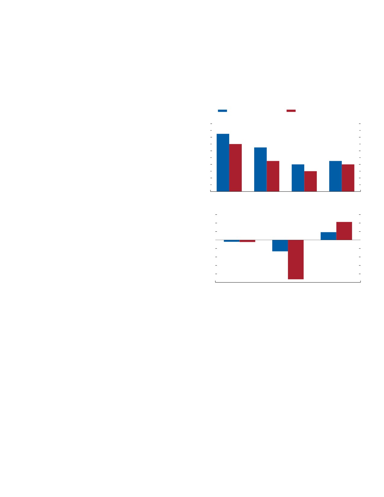
CHAPTER 2 Managing Expectations: Inflation and Monetary Policy

Moreover, the role of fiscal policy for inflation and

Figure 2.14. Policy Objectives, Social Welfare, and

inflation expectations is likely more complex than

Expectations Formation

what can be captured by the illustrative model here. As

After a cost-push shock, the time it takes inflation to get back to target in an

shown in the empirical analysis in Box 2.2, worse fiscal

economy depends on the formation of expectations and the central bank’s

positions (that is, higher public debt and persistent

objectives. A greater share of backward-looking learners in the economy draws

out the timeline, regardless of policy objectives. A comparison with a stylized

deficits) can reduce the effectiveness of sounder mon-

social welfare function suggests that a faster path may come with costs unless

etary policy frameworks in lowering inflation expecta-

driven by less persistent shocks.

tions in emerging market and developing economies.

Heterogeneous-agent model

Rational-expectations model

In other words, more sustainable fiscal positions are

associated with lower average inflation expectations.

1. Years for Inflation to Get Back to Target

Even so, there may be conditions under which fiscal

support measures may help to lower inflation or at

least smooth out a sharp inflationary shock, as seen

in Box 2.3’s analysis of the fiscal relief measures to

offset the energy shock in Europe in 2022. Consumers’

perceived or expected persistence of these measures is

critical to how they affect the path of inflation.

Baseline

Double weight

No weight on

Less persistent

Monetary Policy Faces Inflation-Output Trade-Offs

on inflation

output gap

shock

In the current context in which core inflation

2. Social Welfare versus Baseline

in many countries is more persistent than initially

(Percent difference)

expected, an important question policymakers face is

the timeline for bringing inflation back to target. Tis

subsection illustrates how a central bank’s optimal

-10

choice, one that minimizes a stylized welfare loss

-20

function, would vary with its objectives and the prop-

-30

erties of the underlying shocks in the context of the

-40

illustrative model. Te baseline case assumes that the

-50

central bank seeks to minimize a function that equally

Double weight

No weight on

Less persistent

weights the welfare losses from the output gap and

on inflation

output gap

shock

inflation target deviations, alongside a smoother policy

Source: IMF staff calculations.

rate path.²⁵ In the heterogeneous agents’ model, the

Note: The figure assumes that a cost-push shock raises inflation 2 percentage

central bank under the baseline would opt to calibrate

points above target initially. The shock has an estimated half-life of 14 quarters. In

the baseline scenario, the central bank’s policy seeks to minimize welfare loss, as

the policy rate path to bring inflation back to target in

measured by a stylized social welfare function. The latter includes an interest rate

about four years (Figure 2.14, panel 1).²⁶ If the central

smoothing term and weighs output gap and inflation deviations equally. Panel 2

welfare baselines differ by the expectations formation process. For an identical

bank were to accelerate this process and decided to

welfare function, social welfare is about 20 percent higher with rational than with

double the weight of inflation in its objective function,

heterogenous expectations, reflecting enhanced policy effectiveness and lower

then it would aim for inflation to come back to target

endogenous persistence of shocks. See Online Annex 2.5 for further details on the

assumed objective and social welfare functions and other aspects of the dynamic

in about three years. In a more extreme case in which

stochastic general equilibrium model. The “Less persistent shock” scenario

reduces the half-life of the shock to 6.5 quarters.

²⁵Specifically, the exercise assumes that the central bank minimizes

a welfare loss function that values interest rate smoothing and

equally weights output and inflation deviations (a quadratic loss

the central bank cares only about inflation, it would

function). Te central bank is also assumed to know the expectations

choose to bring inflation back to target in two years.

formation process in the economy and to have full information on

However, this latter choice entails lower welfare if

the path of future cost-push shocks. See Online Annex 2.7 for more

details on the exercise.

society in fact values equally both minimal output gaps

²⁶Since shock persistence is highly uncertain, this subsection

and inflation target deviations (Figure 2.14, panel 2).²⁷

presents two scenarios assuming different degrees of persistence.

If the shock turns out to be less persistent, monetary policy will

be able to bring inflation back to target in less than four years

²⁷Te welfare losses clearly depend on the weights that each soci-

(Figure 2.14, panel 2).

ety would put on inflation target and output gap deviations.

International Monetary Fund | October 2023

WORLD ECONOMIC OUTLOOK: Navigating Global Divergences

Finally, if there were only forward-looking learners in

economy, it could take up to four years to get inflation

the economy, then it would be optimal to bring infla-

back to its target if central banks equally weigh the

tion back to target in about three years. Overall, even

welfare losses from inflation deviating from target with

if the cost-push shock were half as persistent as under

those from output gaps. If central banks were to disre-

the baseline assumptions, it would still be optimal to

gard the output gap effects of their actions and tighten

wait about two years to bring inflation back to target.

more and faster, the analysis suggests they could bring

All these scenarios show that in the presence of a per-

inflation back to target in two years, but at the cost of

sistent cost-push shock and partially backward-looking

lower output.

expectations, it may be optimal to use a more extended

Taken together, the chapter’s results and recent

timeline over which inflation is brought to target.

findings suggest that monetary policymakers benefit

from having a clear understanding of the nature of

expectations processes at play in their economies.

Conclusions

Improved data on expectations could involve close

Near-term inflation expectations rose sharply in

monitoring and enhanced collection of information

many economies amid the economic recovery from the

on expectations across economic agents, particularly

pandemic and after the large cost-push shocks of 2022

near-term expectations which appear more important

(from the surprise rises in energy and commodity prices

for current inflation dynamics. Te performance of a

and supply chain disruptions). Te rise in expectations

novel measure of firms’ inflation expectations derived

was broadly synchronous across professional forecasters,

from text analysis of firms’ earnings calls presented in

financial markets, households, and firms. In contrast,

this chapter points to how technological developments

long-term expectations have remained broadly stable,

have made it more feasible and cost-effective to extract

on average, with no signs of de-anchoring. Past episodes

timely information on expectations.

with jointly rising near- and long-term inflation expecta-

Improvements to monetary policy frameworks—

tions over a sustained period indicate it took about three

particularly those that enhance central bank indepen-

years on average for inflation and near-term expectations

dence and transparency—and communication strategies

to return to pre-episode levels, although there has been

have the scope to boost the share of forward-looking

wide variability across episodes.

learners in the economy and thereby the effectiveness

An estimated hybrid Phillips curve suggests

of monetary policy (Dincer, Eichengreen, and Geraats

that near-term inflation expectations play a more

2022). Recent literature suggests that exposure to news

prominent role in explaining current inflation than

improves the precision of perceptions and expectations,

long-term expectations. Over recent quarters, the driv-

increases confidence, and lowers dispersion of beliefs

ers of inflation have shifted from underlying cost-push

(Lamla and Vinogradov 2019). Haldane, Macaulay, and

shocks toward inflation expectations, particularly

McMahon (2020) recommend that central bank com-

for the average advanced economy. For the average

munications strategies should start with the three Es:

emerging market economy, expectations play a smaller

explanation, engagement, and education. Focusing on

role than lagged inflation, but still a significant one.

household and firms, other recent contributions suggest

Tis is particularly relevant because the pass-through

addressing inattention by taking account of audience

of expectations to inflation increases when inflation is

segmentation and using sources of communication

already elevated, as it is in the present time.

that have been identified as most relevant for people

More generally, the analysis underlines the critical

with more backward-looking expectations—for exam-

role of the expectations formation process for inflation

ple, television in the United States and euro area (see

dynamics and the conduct of monetary policy. With

Coibion and others 2020, D’Acunto and others 2020,

a larger share of backward-looking learners in the econ-

and Weber and others 2022, among others). Tey also

omy, mean expectations are more persistent and can

suggest shaping messages that are simple and repeated

get stuck at a higher level when inflation is higher for

often, investing in financial literacy education, empha-

a sustained period. Tis stickiness reduces the potency

sizing the goal and not the instruments (for example,

of monetary policy and increases the sacrifice ratio (or

former European Central Bank President Mario Draghi’s

cost in terms of output forgone) compared with a case

2012 “whatever it takes” speech), and targeting the mes-

in which expectations are purely forward looking.

sage to the conjuncture. Tese communication strategies

Given the greater inflation persistence implied by

can help economic agents become aware of, understand,

having a share of backward-looking learners in the

and internalize the effects of monetary policy decisions.

International Monetary Fund | October 2023

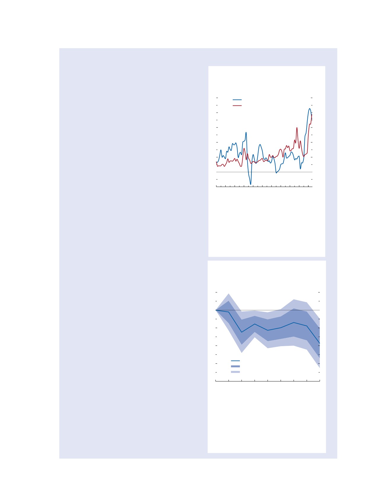
CHAPTER 2 Managing Expectations: Inflation and Monetary Policy

Box 2.1. Firms’ Inflation Expectations, Attention, and Monetary Policy Effectiveness

The inflation expectations channel can improve when

Figure 2.1.1. US Inflation and Firms’

firms pay greater attention to monetary policy and

Attention to the Federal Reserve

develop a stronger understanding of what it means for

(Percent, unless noted otherwise)

their business prospects. However, surveys of firms’ infla-

tion expectations are scarce and time consuming to imple-

2.0

Headline Inflation

ment (Coibion and others 2020). This box introduces a

ECFACB (right scale, index)

new firm-level index of near-term inflation expectations

1.6

based on text analysis of firms’ earnings calls and presents

preliminary findings on how firms’ attention to inflation

1.2

can influence the effectiveness of monetary policy.

0.8

An index of firms’ attention to monetary policy is

built in this box using a text analysis of firms’ earnings

0.4

calls. Details of its construction feature in Albrizio,

Dizioli, and Simon (2023) and are similar to those

0.0

for the firm-level index of inflation expectations, as

described in Online Annex 2.6. Specifically, an index

–2

-0.4

2002

for US firms’ attention to the Federal Reserve is con-

structed based on the frequency of sentences discussing

Sources: NL Analytics; S&P Capital IQ; and IMF staff

monetary policy in their earnings call transcripts (see

calculations.

Note: The figure shows an index of firms’ attention to the

Figure 2.1.1 for an aggregate picture).

central bank (right scale), extracted from earnings call

Dynamic responses are estimated using local pro-

transcripts and actual inflation (left scale). The index is

jections to assess the effect of a monetary policy shock

calculated by applying text-based analysis using transcripts

of US-based companies’ earnings calls and measures the

on a firm’s inflation expectations, conditional on the

intensity of discussion related to the Federal Reserve.

firm’s attentiveness to monetary policy.¹ Attentiveness

ECFACB = Earnings-Calls-based Firm Attention to the

by firm is de-meaned by sectoral average attentiveness

Central Bank index.

in the regression. Because of the de-meaning and

Figure 2.1.2. Role of Attention in Monetary

the inclusion of time fixed effects, the interaction

Policy Effectiveness

between the monetary policy shock and attention

(Percent of ECFIE standard deviation)

reflects the marginal effect of monetary tightening

on a firm’s inflation expectations from its being more

attentive. More attentive firms decrease their infla-

tion expectations by about 1 percent of one standard

deviation more than the average after four quarters

(Figure 2.1.2).² Tis corresponds to an amplification

of about one-fourth to the sector’s average negative

-1

response. Te results bolster the chapter’s argument

that monetary policy is more effective when monetary

-2

policy frameworks and communication strategies help

improve agents’ trust in central banks and their under-

Dynamic response

standing of central banks’ monetary policy decisions.

-3

68 percent confidence interval

90 percent confidence interval

Te authors of this box are Silvia Albrizio, Pedro Vitale

-4

Simon, and Allan Gloe Dizioli.

-1

¹Te specification includes an interaction between a US mone-

Horizon (quarters)

tary policy shock measure (from Acosta 2023) and an attention

index, firm and time fixed effects, and firm-level controls, based

Sources: Haver Analytics; NL Analytics; S&P Capital IQ; S&P

on Ottonello and Windberry (2020). Firm-level controls include

Compustat; and IMF staff calculations.

sales growth, leverage, employment, total assets, and share of cur-

Note: The line in the figure is the estimated cumulative

rent assets in total assets. Standard errors are two-way clustered

impulse response to a one-standard-deviation

by firms and time.

contractionary monetary policy shock for a firm that is one

standard deviation above the average firm attentiveness in

²Te shocks have been scaled to have unit standard deviation.

its sector. Shaded areas represent 68 (outer) and 90 percent

(inner) confidence intervals. ECFIE = Earnings-Calls-based

Firm Inflation Expectations index.

International Monetary Fund | October 2023

INTERNATIONAL MONETARY FUND. Navigating Global Divergences (October 2023) - page 2