Content .. 1 2 3 4 5 ..

Technology of watch production - part 4

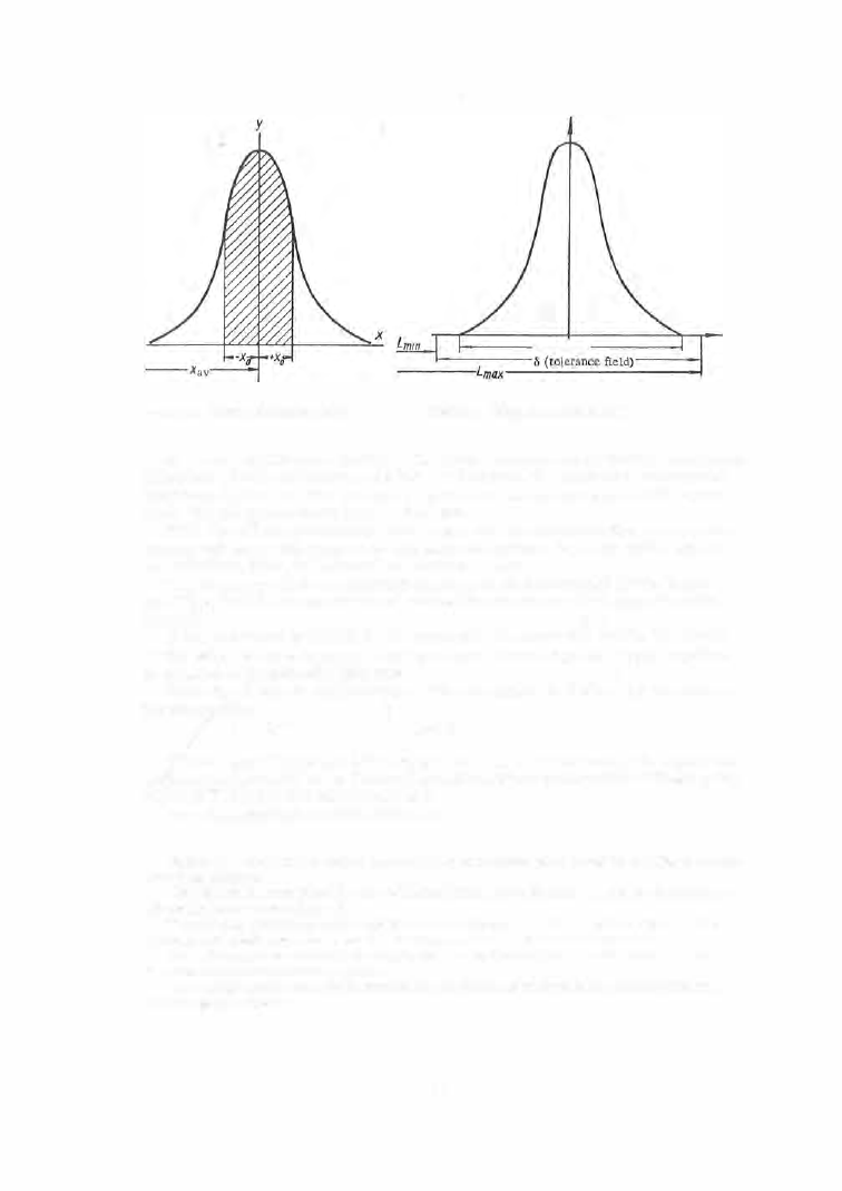
FIGURE 4. Normal distribution curve

(range)

FIGURE 5. Range and tolerance field

Z·o

2 . 4 3 X 0 . 02

0 . 04 8 6 . The total tolerance is 0 . 04 8 6 X 2

�

0 . 1 0 mm .

Allowing a 1 . 5 % reject rate and for

0 . 0 2 m m , the tolerance can b e es tab

l is hed as 0 . 1 0 m m . For the s ame value o f

, and allowing a 0 . 2 7 o/o reject

rate, the toler ance m us t b e 6

0 . 1 2 m m .

With the aid of dis tribution curves one can characterize the process a c

curacy n o t only with res pect t o dimens ional errors , but als o with res pect

to deviations from the correct geometrical s hape .

The accuracy o f the technological process is determined by the bas ic

condition that the range m us t not exceed the tolerance field (s pecification

limi ts ).

If the c ondition is fulfilled, the work will be c onducted within the limits

of the es tablis hed tolerance , and therefore without rejects . This condition

is pres ented graphically in Figure 5 .

Since the range is 6cr, production without rejects is defined by the follow

ing inequality:

6o<�.

If this inequality is not fulfilled Q. nd

6o > a,

it is necess ary to replan the

engineering process or to envis age s upplementary process ing of thos e parts

which fall outs ide the tolerance fiel d .

W e will cons ider s everal examples .

Example 1.

Parts from two batches, produced by the same technological process but at different machine

settings are measured.

The distribution curves plotted for the two batches v1ill be roughly identical, but will be displaced from

one another by the value a (Figure 6).

When w orking with holding and locating fixtures, the shift can be explained only by a difference in the

positions of the working parts of the machine, the clamping devices and tools for the two cases.

If we plot a curve for a mixed batch of parts, processed by different reamers, different punches, etc. ,

the curve will have two summits (Figure 7).

The multiple-summit curve can be considerei:l as the summation of curves having different arithmetic

means (population means).

1 3

If the various groups of parts are machined by different processes, the individual distribution curves,

which together form the common multiple-summit distribution curve , may also differ in shape .

Example 2,

Assume that a batch of parts manufactured by an invariable process using locating fixtures

has been measured, The distribution curve is plotted and superimposed on the tolerance field. The range is

seen to be smaller in absolute value than the tolerance field (Figure

8),

but since the population means is

displaced to the right, rejects will result.

The proportion of rejects ( as a percentage of the total number of parts in the batch) is represented by the

hatched area of the curve.

The following conclusions can be drawn on the basis of the curve obtained.
The process adopted can reliably produce work without rejects, since

e = 6a<a.

The fact that rejects are obtained is due to the shift of the population mean relative to the tolerance field.
In order to produce work without rejects, all that is necessary is to readjust the machines.

Example 3,

rt is required to select from among three possible technological processes the one ensuring

maximum accuracy.

Three groups of parts are experimentally machined using the three processes, and after measuring the

parts the standard deviation for each group is calculated.

The process which gives the smallest value for

will be ensuring the highest accuracy.

Having investigated a process by m eans of distribution curves, conclu

s ions can b e drawn concerning its accuracy under given processing condi

tions . On the basis of thes e data, specifications for the accuracy of the

various technological processes can be established.

Using thes e specifications, engineers can correctly s elect the process

giving the required accuracy.

FIGURE 6. Normal distribution curves with
different positions of the population mean

FIGURE

Two-summit distribution curve

The influence of individual factors on the process accuracy can be inves

tigated with  the  aid  of  the  distribution  c urves .  The  factor in  question  is
varied,  keeping the  remaining parameters  of  the  process  unchanged .   The
comparison of the  distribution  curves  obtained before and after the  variation

indicates that the m ethod of determination of process accuracy by means of

distribution curves is of general applicability and makes it possible to find

methods f or increasing process accuracy.

The bas ic m ethods for increasing the machining accuracy in watch pro

duction are:

1 . Increasing the durability of the tool , thus achieving increas ed s tability

in the machined dimensions .

2 . Reducing the range of the variation in the mechanical p roperties of

the m etal us ed.

3 .

Machining the important s urfaces of the part in one hold .

4 . Combining the des ign and reference s urfaces and us ing o n e s ingle

s urface as a bas e for the various operations .

'P(range)

(tolerance

FIGURE 8.

Distribution curve for work produced

by improperly adjusted machine

Average economic accuracy.

Each machining process has a definite

accuracy under normal production conditions . On the bas is of numerous

obs ervations , the accuracy of the various machining process es has been

es tablis hed and is called the a v e r a g e e co n o m i c a c c u r a c y .

e average economic accuracy is the accuracy achievable under normal

pro duction conditions , that is , when the machines have the s pecified accu

racy, the fixtures and tools corres pond to the drawings and s pecifications,

the work is carried out as s pecified, and the pers onnel have the required

qualifications .

Data on the average economic accuracy in watch manufacturing are

given in Table 2 .

TABLE

2°

Average economic process accuracy in 1vatch manufacturing

Process

Turning on Swiss-type automatic screw machines

a) bar diameter up to 6 mm :

for diameter

•

for length

•

b) diameter from 6 to 1 0 mm :

for diameter

•

for length

•

c) diameter from

to 16 mm:

for diameter

•

for length

•

Based on data from watch plants.

1 5

Average economic pro

cess accuracy, mm

0.005- 0.010
0.010-0.020

0.01 0-0.020
0.02 0-0.030

0.01 5- 0.025
0.030- 0.050

Process

Facin g and counterboring flat watch parts on the S -57M, S-81A,

S-175, S-178 machines, etc . :

for diameter

•

for depth

•

Milling gears and pinions on the S-40 and 530A machines, on the

the ex ternal diameter :

module 0,1 5 mm

•

0.15 to 0.30 mm

•

0.30 to 0.50 mm

•

M illing recesses in flat brass parts on the S-50, S-187, S -210

machines, etc. :

for depth- area up t o 5 0 mm2

•

for depth- area more than 50 mm2

•

for contour

•

. •

•

• •

. •

•

Drilling hol es :

diameter up to 1 mm

•

diameter from 1 to 3 mm

•

R eaming holes :

diameter up to 1 mm

diameter from 1 to 3 mm

. .

. •

•

Shaving holes:

diameter up to 3 mm

•

diameter from 3 to 7 mm

•

Stamping

Blanking:

a) blanks of siz e up to 25 mm and thickness up to 2 mm

b) blanks of siz e larger than 25 mm and thickness more than

2 mm

•

• • •

•

• ·

• · •

• • •

Shaving

a) parts of siz e up to 25 mm and thickness up to

•

b) partS of siz e larger than 25 mm and thickness more than

2 mm

•

Combined blanking and shaving:

a) parts of siz e up to 25 mm and thickness up to 2 mm . . . .

b) parts of siz e larger than 25 mm and thickness more than

2 mm

•

Rol ling and dr awing

•

Cylindrical grinding :

diameter up to 1 mm

•

diameter from 1 to 3 mm .

. .

diameter from 3 to 1 0 mm

•

Surface grinding (t hickness):

area up to 5 mm2 . . . . . . . . . . . . . . . . . . . . . .

area from 5 to 50 mm2

. .

. ,

. .

•

area more than 50 mm2

Circular polishing :

diameter up to 1 mm
diameter from 1 to 3 mm . .

diameter from 3 to 1 0 mm

•

Plane polishing:

area up to 5 mm2

•

area from 5 to 50 mm2 . . . . . . . . . . . . . . . . . . .

TABLE 2 ( cont' d)

Average economic pro

cess accuracy, mm

0.02 Q- 0.050

O , O l Q- 0,030

0,01Q -0,025
0.015- 0.035
0.03Q- 0,050

O , O l Q- 0,025

0.02 Q- 0.030
0.02 0- 0.050

0.008- 0.015
0.015- 0.030

0.005- 0.010

0.008 -0.015

0.005-0.010

0.01 Q-0,020

0.02 Q- 0,050

0.05Q-0,150

O . O lo- 0.020

0.02 Q- 0,050

0.01 5- 0.030

0.030-0.1 00

0.01Q- 0,050

O . Ol Q- 0.015

0 .015- 0.020
0,02 Q- 0,025

O . O l Q- 0.020

0.02 Q-0.030
0.03Q- 0,050

0.005 -0.010

O . O lo- 0.015

0.015- 0.020

0.02 Q -0.030

0.03 Q -0,050

Content .. 1 2 3 4 5 ..