MANUAL OF NATO SAFETY PRINCIPLES FOR THE STORAGE OF MILITARY AMMUNITION AND EXPLOSIVES (May 2010) - page 17

NATO/PFP UNCLASSIFIED
AASTP-1
(Edition 1)
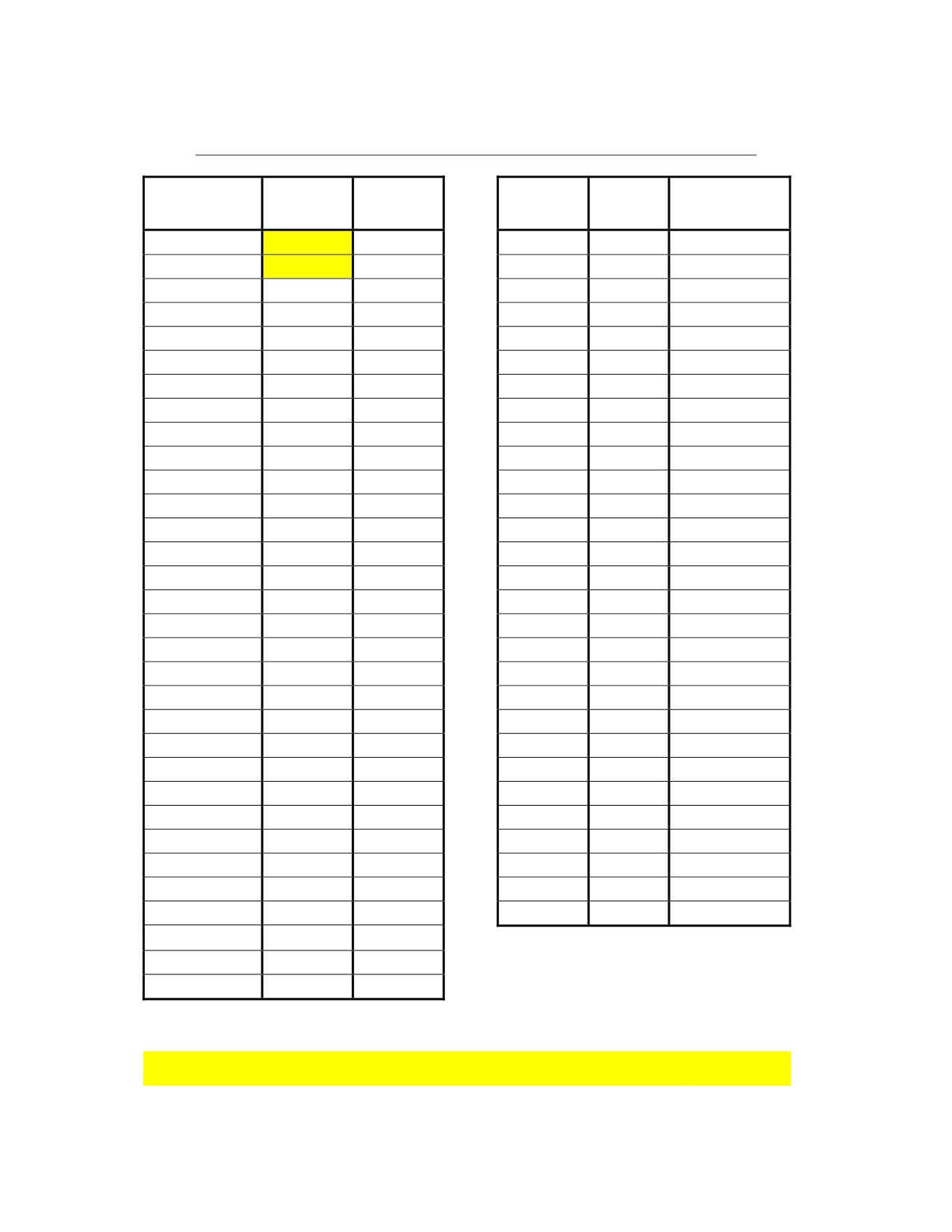
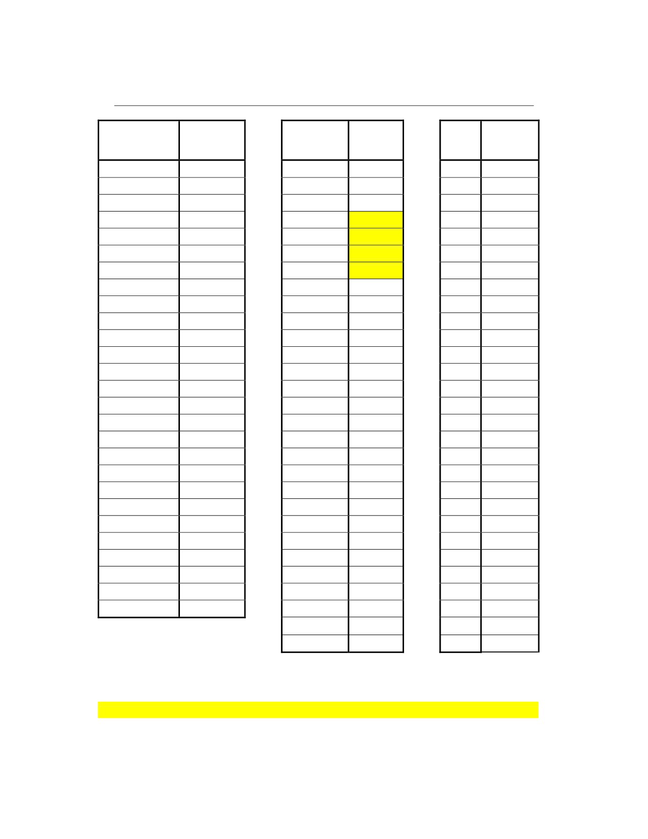
Do values for typical x (= A + B x Ro/fp ) values are given in the
table in Figure 3-XIV.
c)
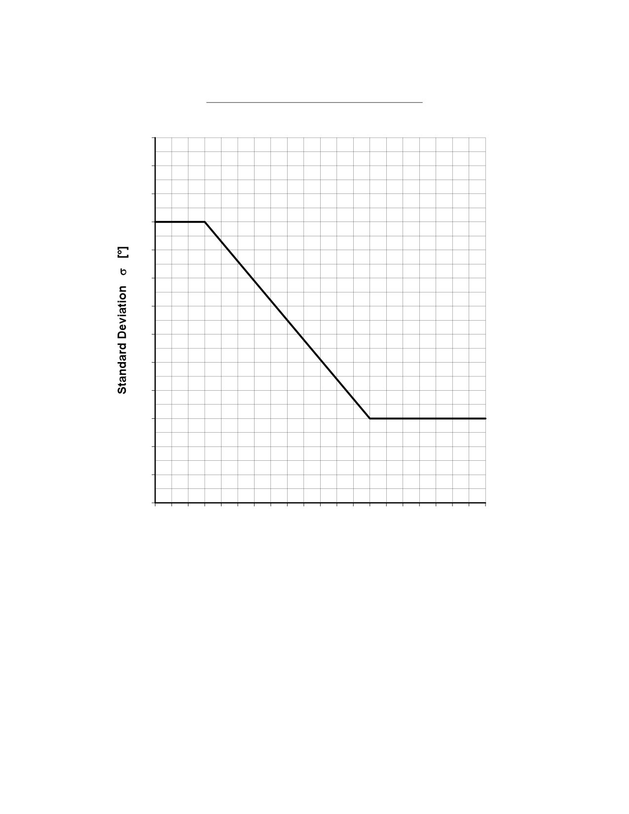
Calculate the standard deviation σ according to Figure
3-XIII.
Typical values for σ as a function of the la/da ratio are given in
Figure 3-XII.
d)
Calculate the corresponding α and Rs values for each Do value
(Figure 3-IX).
⎛0.0179
⎞
2
α =
−2
⋅
ln⎜
⎟
⋅
σ
⎜
⎟
D
⎝
0
⎠
ln(x) values for typical x =
0.0179 / Do values are given in the table
in Figure 3-XIV.
Rs = Ro x tan(α)
tan(α) values for typical α values are given in the table in Figure 3-
XIV.
e)
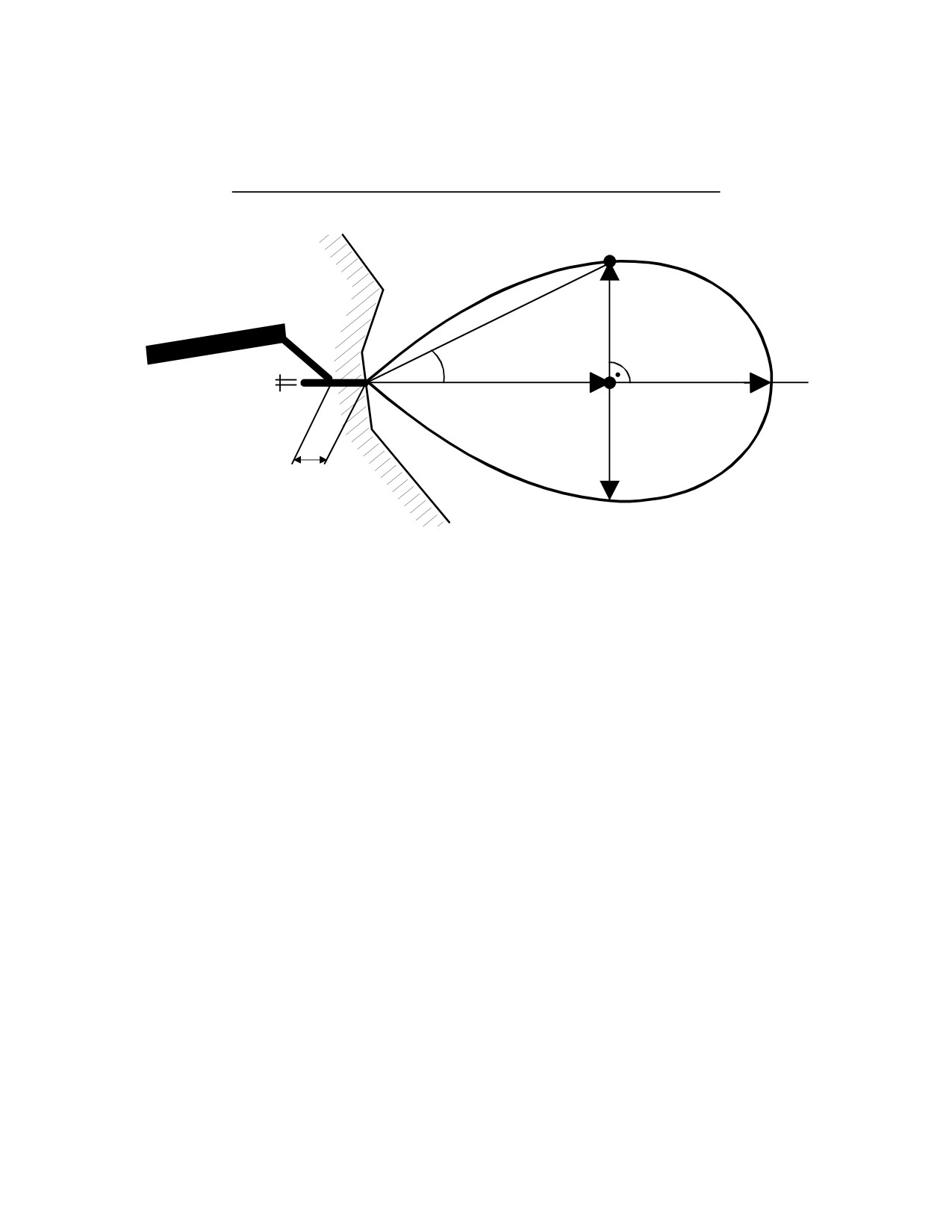
Each related combination of Ro and Rs defines a point D on the IBD
contour line were the debris density is one hazardous fragment
(energy greater than 79 Joules) per 56 m2. Therefore, drawing a
line starting and ending at the adit portal and connecting all the
previously calculated points D (and Ro max) establishes the IBD
contour line.
Example
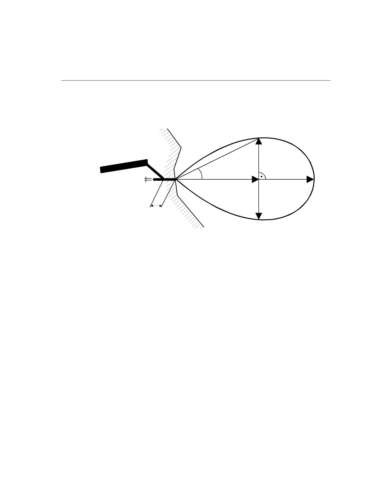
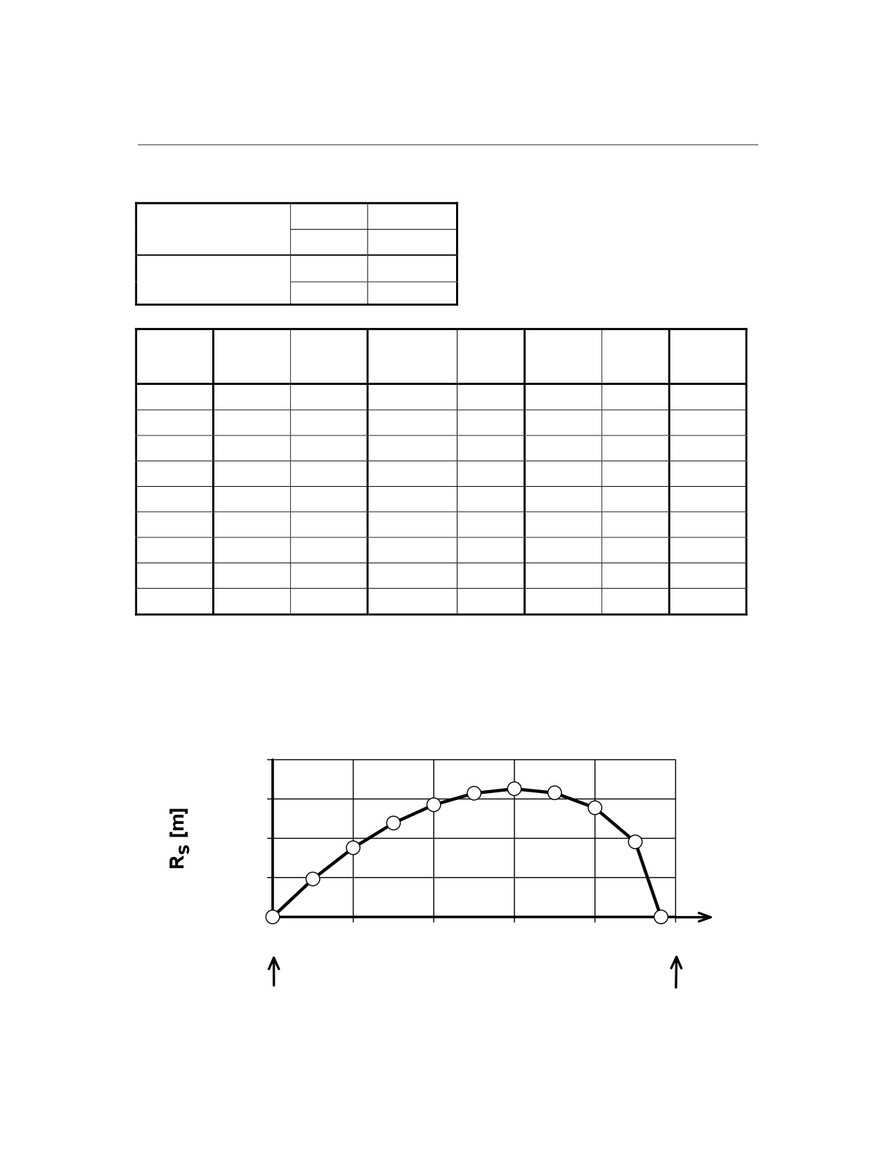
A typical example how to calculate an IBD contour line is given in
Figure 3-XVa and 3-XVb.
Special Cases
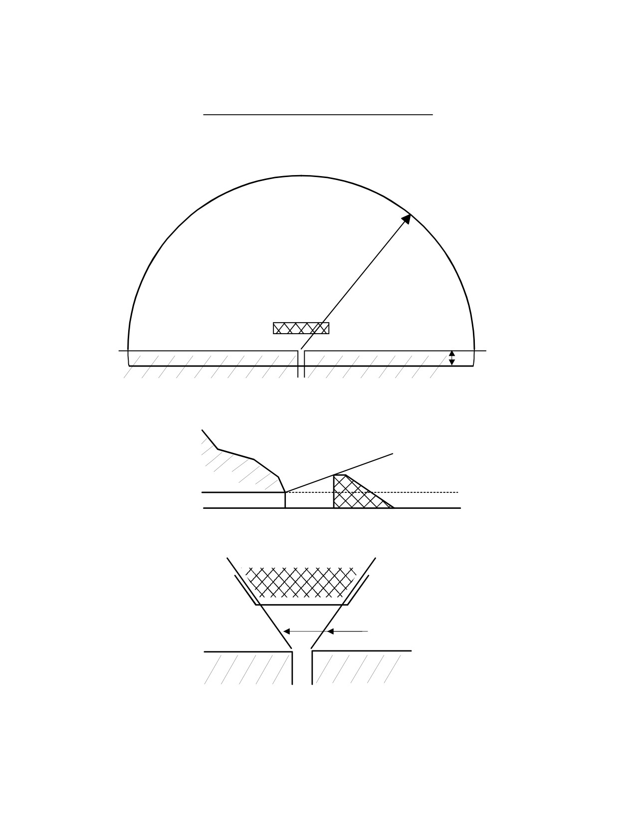
Barricade in Front of the Adit Portal
a) If an artificial or natural barricade is located within 10 to 20 m from
the portal, and if all of the following conditions for an effective
barricade are met, the form of the IBD contour line approaches a
semicircle according to Figure 3-XVI.
b) Conditions for effective barricades are:
- The front facing the portal must be more or less vertical
NATO/PFP UNCLASSIFIED
-III-3-22-
Change 3

NATO/PFP UNCLASSIFIED
AASTP-1
(Edition 1)
- The front facing the portal must be normal to the extended adit
axis
- The barricade must be symmetrical to the extended adit axis
- It has to withstand the expected explosion effects
- The width of the barricade has to "cover" the IBD contour line as
calculated according to Chapter 1.3 to the side of the portal
(Figure 3-XVI, Ground Plan)
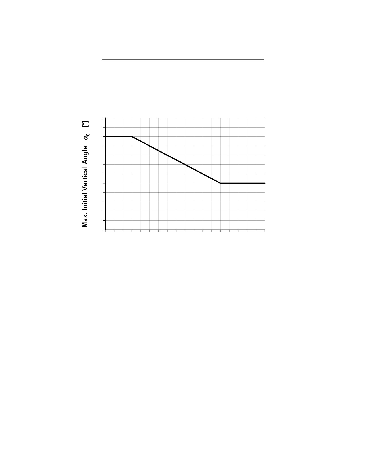
- The height of the barricade has to "cover" at least half of the
maximum initial vertical launch angle according to Figure 3-XVII
(Figure 3-XVI, Section).
c)
If the conditions for an effective barricade are met, the maximum
range Ro max of the IBD contour line can be calculated according to
Chapter 1.3. However, regardless of the la/da ratio, the portal
parameter fp is always to be set as 0.4 for installations with an
effective barricade. The IBD contour line is a semicircle in front of
the adit portal with the centre at the adit portal. The IBD contour
line also extends a short distance backwards as indicated in Figure
3-XVI.
d)
If the conditions for an effective barricade are not met, the debris
distribution may vary considerably. Therefore, only a conservative
approach for the calculation of the IBD contour line can be given in
this manual.
In such cases the IBD contour lines for adits with an effective
barricade and adits without a barricade in front of the portal have to
be calculated and superimposed. Exposed objects must be outside
of both IBD contour lines.
Further information about the effects of barricades that are only
partially effective and especially barricades that are oblique to the
extended adit axes is given in AASTP-4 and [2, 3, 6].
e)
In addition to barricades located near the adit portal also hills and
mountains farther away may limit adit debris throw. In cases where
the application of the standard IBD contour line leads to major
restrictions, effects of such natural obstacles may be taken into
account. However, further information about the influence of the
topography on adit debris throw and a relatively complicated
calculation procedure are only given in AASTP-4.
Storage Chambers with Very Short Adits
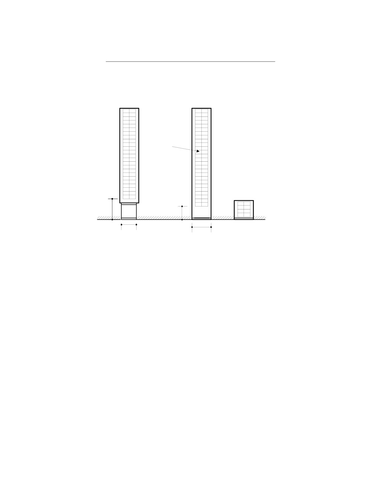
a) At installations with a very short adit, the relevant length of the adit
section just behind the portal (la) is to be measured from the portal
to the first ammunition stack (Figure 3-XVIII).
NATO/PFP UNCLASSIFIED
-III-3-23-
Change 3

NATO/PFP UNCLASSIFIED
AASTP-1
(Edition 1)
b)
If the ratio la/da in this case is 2 or larger, the IBD contour line can
be calculated according to Chapter 1.3.
c)
If the ratio la/da is smaller than 2, the following two cases have to be
distinguished:
• For very short chambers and ammunition stacks reaching the
portal (Figure 3-XVIII), the IBD contour line is to be calculated as
for an installation with an effective barricade in front of the adit
portal, according to Chapter 1.5.1 and Figure VIII.
• In all other cases, as a conservative approach, the IBD contour
lines for adits with an effective barricade (according to Chapter
1.5.1 and Figure 3-XVI) and adits without a barricade in front of
the portal (according to Chapter 1.3) have to be calculated and
superimposed. Exposed objects must be outside of both IBD
contour lines.
Further information about the effects from explosions in chambers
with short adits is given in AASTP-4 and [2, 3, 6]
Installations with more than one Adit Portal
a) In certain cases storage chambers may have more than one adit or
an adit may have more than one portal, e.g. as a special protection
measure against enemy attacks. In addition, such adits may have
different cross-section areas and the adit axis may point in different
directions.
b) As a general conservative rule, for IBD purposes, the IBD contour
lines as calculated above for the various cases have to be applied
to each adit portal.
c) In cases where the procedure according to b) leads to major
restrictions, a procedure described in AASTP-4 might be used to
take into account further effects, leading - depending on the actual
situation - to corresponding reductions of the IBD contour lines.
Debris Mitigation Measures
a) Debris throw from underground installations on rock is a significant
threat to exposed persons outside and installation. Therefore,
whenever reasonable, measures should be taken to reduce debris
throw. However, if constructional measures are taken, they have to
be designed appropriately to withstand the explosion effects. Be
NATO/PFP UNCLASSIFIED
-III-3-24-
Change 3

NATO/PFP UNCLASSIFIED
AASTP-1
(Edition 1)
aware that failing installation parts may contribute to the debris
throw and even enhance the hazard.
b)
Blast closures according to Chapter 3.2.4.4 and especially the so-
called Klotz-Device are very effective means to reduce not only the
air blast from underground installations but also the debris throw
from the adits. Information about possible reductions achievable
with such devices is given in AASTP-4.
c)
Apart from barricades and self-closing devices (see Chapter 3.2.4.4
and Figure 2-III), there are also other elements reducing adit debris
throw such as blind tunnels and expansion chambers in the adit. In
general, a combination of such elements, especially with a self-
closing device, enhances the mitigation effect.
However, currently there are no models available taking such
mitigation measures in the adit into account (except for the Klotz-
Device). Therefore, the effectiveness of such elements has to be
tested in models with an appropriate scale or with computer
simulations.
Range of Validity and Background Information
a)
Special caution has to be applied if this adit debris throw model is
used outside the range of validity indicated below:
- explosives quantity NEQ:
100 - 500'000 kg
- chamber loading density γc :
1 - 100 kg/m3
- system loading density γs :
0.3 - 100 kg/m3
The chamber respectively system loading density
(γc
/ γs
) is
defined as the ratio between the NEQ and the storage chamber
volume respectively the system volume (chamber volume and adit
volume).
For applications below the lower limits, the model usually
overestimates the debris throw
(IBD is conservative). This is
especially true for storage chambers with very low loading densities
in combination with very long adit tunnel systems with many bends
and other mitigation measures. In such cases the hazard from adit
debris throw may be much lower than indicated by the model
above. To establish reliable adit debris IDB for such cases
appropriate model or full-scale tests are necessary.
No such statement is possible for applications above the upper
limits.
NATO/PFP UNCLASSIFIED
-III-3-25-
Change 3

NATO/PFP UNCLASSIFIED
AASTP-1
(Edition 1)
b) The technical basis for the figures and formulas is mainly derived
from the following report (for additional background information see
[37 - 42]):
NATO - AC/258 Storage Sub-Group - UGSWG
Debris Throw from Adits of Underground Installations in Rock
Basics for Risk Analysis
Technical Background
TM 174-9 // AC/258 CH(ST) IWP 024-02, 30 March 2002
NATO/PFP UNCLASSIFIED
-III-3-26-
Change 3
NATO/PFP UNCLASSIFIED
AASTP-1
(Edition 1)
Figure 3-IX:
General Shape of the Adit Debris IBD Line
IBD Contour
D
Line
Rs
Q
α
R0
R0 max
da
Extended
D0
Adit Axis
la
Rs
Q
: Explosives weight (NEQ)
[kg]
la
: Relevant length of the adit section behind the portal
[m]
da
: Average equivalent diameter of la
[m]
R0
: Distance (range) on the extended adit axis from the portal
[m]
R0 max
: Maximum distance (range) of IBD
[m]
Rs
: Distance (range) to the side of the extended adit axis at R0
[m]
D
: Point on IBD contour line (debris density 1 hazardous fragment per 56 m2) [#/m2]
D0
: Reference value (debris density at R0)
[#/m2]
α
: Angle showing the deviation of D from the extended adit axis
[°]
α = arctan (Rs/R0)
NATO/PFP UNCLASSIFIED
-III-3-27-
Change 3
NATO/PFP UNCLASSIFIED
AASTP-1
(Edition 1)
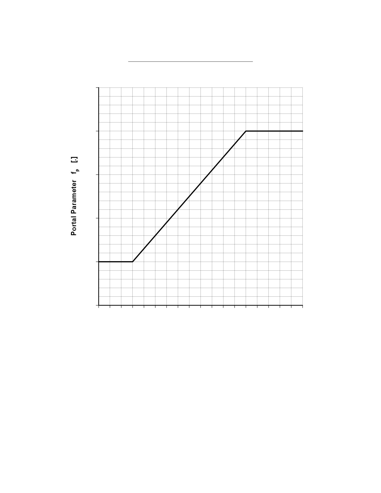
Figure 3-X:
Portal Parameter fp
1.1
1.0
0.9
0.8
0.7
0.6
2
5
7
9
11
13
15
17
20
la/da-Ratio
[.]
fp = 0.7
for
la/da ≤ 5
(wide debris zones)
fp = 0.55 + 0.03 x la/da
for
5 < la/da < 15
fp = 1.0
for
la/da ≥ 15
(narrow debris zones)
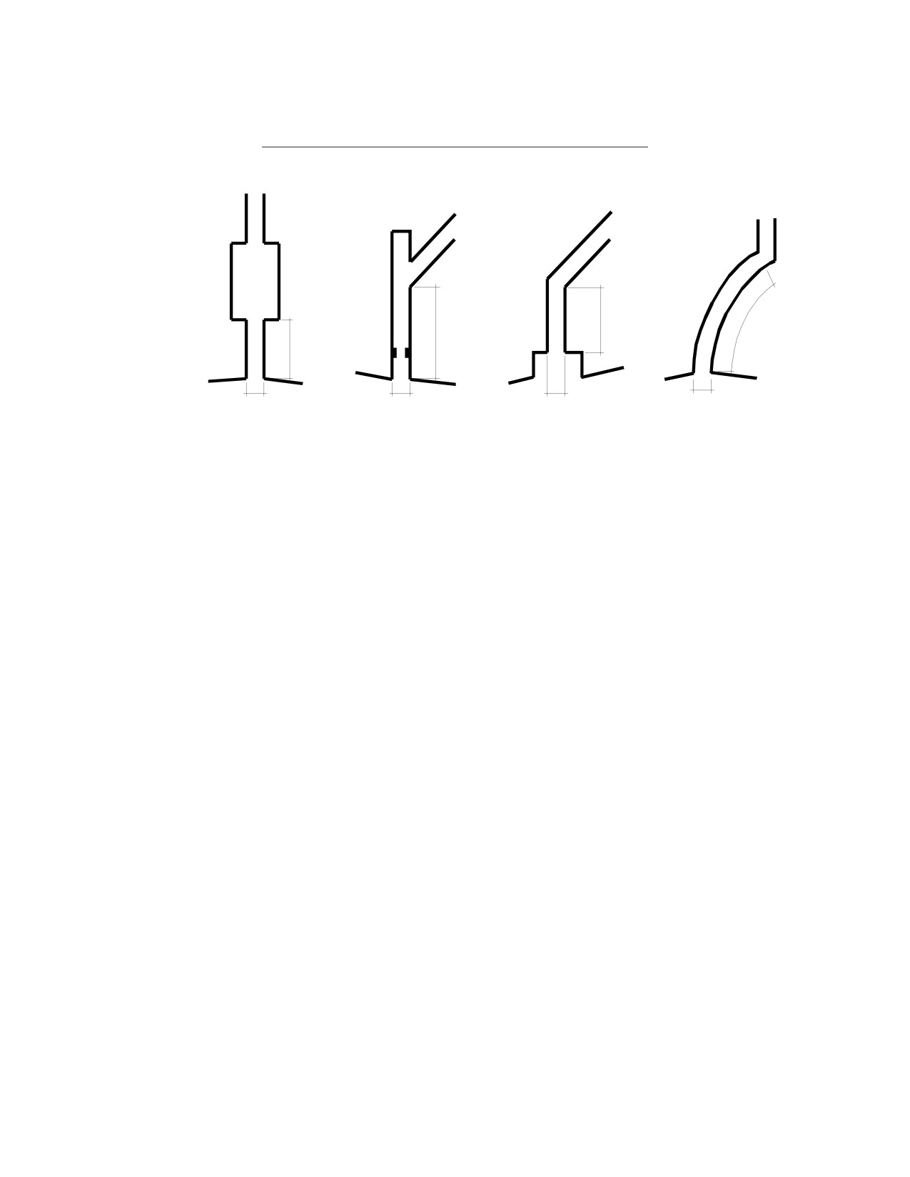
la:
Relevant length of the straight adit section just behind the portal [m]
da:
Average equivalent adit diameter of la
[m]
(da = (4 x Fa / π)0.5)
Fa:
Average cross-section of la
[m2]
NATO/PFP UNCLASSIFIED
-III-3-28-
Change 3
NATO/PFP UNCLASSIFIED
AASTP-1
(Edition 1)
Figure 3-XI:
Determination of the la/da-Ratio
la
la
la
la
da
da
da
da
NATO/PFP UNCLASSIFIED
-III-3-29-
Change 3
NATO/PFP UNCLASSIFIED
AASTP-1
(Edition 1)
Figure 3-XII:
Auxiliary Tables for the Calculation of A, B, fp and σ
NEQ
A
B
la/da-Ratio
fp
σ
[kg]
[.]
[.]
[.]
[.]
[°]
100
-0.645
-0.0335
2.0
0.700
12.0
200
0.0483
-0.0262
3.0
0.700
12.0
300
0.454
-0.0229
4.0
0.700
12.0
400
0.741
-0.0210
5.0
0.700
12.0
500
0.965
-0.0197
5.5
0.715
11.7
600
1.15
-0.0187
6.0
0.730
11.3
700
1.30
-0.0179
6.5
0.745
11.0
800
1.43
-0.0173
7.0
0.760
10.6
900
1.55
-0.0168
7.5
0.775
10.3
1'000
1.66
-0.0164
8.0
0.790
9.90
2'000
2.35
-0.0141
8.5
0.805
9.55
3'000
2.76
-0.0131
9.0
0.820
9.20
4'000
3.04
-0.0125
9.5
0.835
8.85
5'000
3.27
-0.0120
10.0
0.850
8.50
6'000
3.45
-0.0117
10.5
0.865
8.15
7'000
3.60
-0.0115
11.0
0.880
7.80
8'000
3.74
-0.0113
11.5
0.895
7.45
9'000
3.85
-0.0111
12.0
0.910
7.10
10'000
3.96
-0.0110
12.5
0.925
6.75
20'000
4.65
-0.0103
13.0
0.940
6.40
30'000
5.06
-0.00994
13.5
0.955
6.05
40'000
5.35
-0.00975
14.0
0.970
5.70
50'000
5.57
-0.00962
14.5
0.985
5.35
60'000
5.75
-0.00952
15.0
1.00
5.00
70'000
5.91
-0.00944
16.0
1.00
5.00
80'000
6.04
-0.00938
17.0
1.00
5.00
90'000
6.16
-0.00933
18.0
1.00
5.00
100'000
6.26
-0.00929
19.0
1.00
5.00
200'000
6.96
-0.00906
> 20.0
1.00
5.00
300'000
7.36
-0.00896
400'000
7.65
-0.00890
500'000
7.87
-0.00885
Linear interpolation between values is permitted; but
it may lead to deviations of up to
3%,
compared to the real values calculated with the corresponding formula
(for NEQ < 300 kg, the deviation of interpolation of parameter A is even larger)
NATO/PFP UNCLASSIFIED
-III-3-30-
Change 3
NATO/PFP UNCLASSIFIED
AASTP-1
(Edition 1)
Figure 3-XIII:
Standard Deviation σ
15
14
13
12
11
10
9
8
7
6
5
4
3
2
2
3
4
5
6
7
8
9
10 11 12 13 14
15
16
17
18
19
20
21
22
l
[.]
a/da-Ratio
σ = 12
for
la/da ≤ 5
(wide debris zones)
σ = 15.5 - 0.7 x la/da
for
5 < la/da < 15
σ = 5
for
la/da ≥ 15
(narrow debris zones)
la:
Relevant length of the straight adit section just behind the portal [m]
da:
Average equivalent adit diameter of la
[m]
(da = (4 x Fa / π)0.5)
Fa:
Average cross-section of la
[m2]
NATO/PFP UNCLASSIFIED
-III-3-31-
Change 3
NATO/PFP UNCLASSIFIED
AASTP-1
(Edition 1)
Figure 3-XIV:
Auxiliary Tables for the Calculation of D0, ln (x) and tan (α)
x =
D0 = e x
x =
ln (x)
α
tan (α)
A + B x R0 / fp
[pieces/m2]
0.0179 / D0
[.]
[°]
-6.0
0.00248
7.5
2.015
0
0.0000
-5.5
0.00409
5.0
1.609
2
0.0349
-5.0
0.00674
3.0
1.099
4
0.0699
-4.5
0.0111
2.0
0.693
6
0.1051
-4.0
0.0183
1.0
0.000
8
0.1405
-3.5
0.0302
0.75
-0.288
10
0.1763
-3.0
0.0498
0.50
-0.693
12
0.2126
-2.5
0.0821
0.30
-1.204
14
0.2493
-2.0
0.1353
0.20
-1.609
16
0.2867
-1.5
0.2231
0.10
-2.303
18
0.3249
-1.0
0.3679
0.075
-2.590
20
0.3640
-0.5
0.6065
0.050
-2.996
22
0.4040
0.0
1.000
0.030
-3.507
24
0.4452
0.5
1.649
0.020
-3.912
26
0.4877
1.0
2.718
0.010
-4.605
28
0.5317
1.5
4.482
0.0075
-4.893
30
0.5774
2.0
7.389
0.0050
-5.298
32
0.6249
2.5
12.18
0.0030
-5.809
34
0.6745
3.0
20.09
0.0020
-6.215
36
0.7265
3.5
33.12
0.0010
-6.908
38
0.7813
4.0
54.60
0.00075
-7.195
40
0.8391
4.5
90.02
0.00050
-7.601
42
0.9004
5.0
148.4
0.00030
-8.112
46
1.036
5.5
244.7
0.00020
-8.517
48
1.111
6.0
403.4
0.00010
-9.210
50
1.192
6.5
665.1
0.000075
-9.498
52
1.280
7.0
1097
0.000050
-9.903
54
1.376
0.000030
-10.41
58
1.600
0.000020
-10.82
60
1.732
Linear interpolation
between
values is
permitted; but it may lead to
deviations of
up to 3%,
compared to the real values calculated with the corresponding formulas
(for the natural logarithm close to x=1, the deviation of interpolation is even larger)
NATO/PFP UNCLASSIFIED
-III-3-32-
Change 3
NATO/PFP UNCLASSIFIED
AASTP-1
(Edition 1)
Figure 3-XVa:
How to Calculate an IBD Contour Line for Adit Debris - Example
Given:
Debris Density
D = 1 hazardous fragment / 56m2
Rs
α
R0
R0 max
da
Extended
D0
Adit Axis
la
Rs
Clover
Leaf
Shape
Q
= 200'000 kg TNT
la
= 32 m, da = 4 m
=>
la/da = 8
Wanted: IBD Contour Line (where Debris Density D = 1 Hazardous Piece per 56 m2 [#/m2])
Solution: 1)
R0 max on the extended adit axis:
Portal Parameter (1.2 d) - Figure II or IV)
fp
=
0.790
Parameter A (1.3 a) - Figure IV)
A
=
6.96
Parameter B (1.3 a) - Figure IV)
B
=
-0.00906
R0 max = fp x (-4.025 - A) / B = 958 m
2)
R0 (<Rmax) on the axis and the corresponding Rs normal to the side:
To determine the clover leaf shaped contour of the debris zone with a density of D =
1 haz-#/56m2, R0 and the corresponding Rs have to be calculated an appropriate
number of times (starting with Rmax and ending at the portal)
Example:
R0 = 500 m
Debris Density at R0 (1.3 b) - Figure VI)
D0
=
3.41 #/m2
Standard Deviation (1.3 c) - Figure IV or V)
σ
=
9.90°
Deviation from the axis (1.3 d) - Figure VI)
α
=
32.09°
α = (-2 x ln(D/D0) x σ2)0.5
Rs = R0 x tan(α) = 313 m for R0 = 500 m
NATO/PFP UNCLASSIFIED
-III-3-33-
Change 3
NATO/PFP UNCLASSIFIED
AASTP-1
(Edition 1)
Figure 3-XVb:
How to Calculate an IBD Contour Line for Adit Debris - Example
NEQ [kg] 200'000
A [.]
6.96
B [.]
-0.00906
la / da [.]
8
fp [.]
0.790
σ [°]
9.90
R0
x =
D0 = e x
x =
ln (x)
α
Rs
tan (α)
[m]
A+BxR0/fp
[#/m2]
(1/56)/D0
[.]
[°]
[m]
900
-3.362
0.0347
0.515
-0.664
11.4
0.2018
182
800
-2.215
0.109
0.164
-1.811
18.8
0.3412
273
700
-1.068
0.344
0.0519
-2.958
24.1
0.4469
313
600
0.0790
1.082
0.0165
-4.104
28.4
0.5399
324
500
1.226
3.407
0.00524
-5.251
32.1
0.6269
313
400
2.373
10.73
0.00166
-6.398
35.4
0.7110
284
300
3.519
33.77
0.000529
-7.545
38.5
0.7942
238
200
4.666
106.3
0.000168
-8.692
41.3
0.8778
176
100
5.813
334.7
0.0000534
-9.839
43.9
0.9628
96
IBD Contour Line
(other side symmetrical)
400
300
200
100
Extended
Adit Axis
0
0
200
400
600
800
1000
R0 [m]
Adit Portal
R0 max
NATO/PFP UNCLASSIFIED
-III-3-34-
Change 3
NATO/PFP UNCLASSIFIED
AASTP-1
(Edition 1)
Figure 3-XVI:
Influence of a Barricade
IBD Contour Line
R = R0 max
Barricade
Portal
0.1 x R0 max
Adit
Section
α0 / 2
Adit Portal
Barricade
Ground
IBD Contour Line
Plan
without Barricade
Portal
NATO/PFP UNCLASSIFIED
-III-3-35-
Change 3
NATO/PFP UNCLASSIFIED
AASTP-1
(Edition 1)
Figure 3-XVII:
Maximum Initial Vertical Angle α0
60
55
50
45
40
35
30
25
20
15
10
5
0
2
5
7
9
11
13
15
17
20
la/da-Ratio
[.]
α0 = 50°
for
la/da ≤ 5
(wide debris zones)
α0 = 62.5° - 2.5° x (la/da)
for
5 < la/da < 15
α0 = 25°
for
la/da ≥ 15
(narrow debris zones)
la
:
Relevant length of the straight adit section just
behind the portal
[m]
da
:
Average equivalent adit diameter of la
[m]
(da = (4 x Fa / π)0.5)
Fa
:
Average cross-section of la
[m2]
NATO/PFP UNCLASSIFIED
-III-3-36-
Change 3
NATO/PFP UNCLASSIFIED
AASTP-1
(Edition 1)
Figure 3-XVIII:
Installations with Very Short Adits
Ammunition
stacks
Very short
chamber
la
la
da
da
NATO/PFP UNCLASSIFIED
-III-3-37-
Change 3

NATO/PFP UNCLASSIFIED
AASTP-1
(Edition 1)
Debris from Nearby, Failed Structures:
The dynamics of this debris will be highly dependent on site-specific
parameters. Site-specific analyses should be done when this type
of debris is of concern.
Debris Arising from Failure of Cover, Crater Debris [18-22, 34]
a)
The chamber cover thickness is the shortest distance between the
natural rock surface at the chamber ceiling (or in some cases, a
chamber wall) and the ground surface. If the cover consists of part
rock and part soil, the effective thickness of the cover is determined
based on mass. A conservative estimate is to treat soil as having
one-half the mass of rock. Therefore, 10 m of rock and 2 m of soil,
with one-half the density of the rock, equals 11 m of equivalent rock
cover. If the percentage of soil to rock exceeds 20% a site-specific
analysis should be conducted.
Unless the cover is adequate, an underground explosion will cause
breaching of the cover. Rock, and to a lesser degree structural
material, is projected as debris in all directions from the breached
cover into the surroundings.
The hazard from this type of debris depends on the quantity of
explosives
(Q) involved, the scaled cover depth
(C/Q1/3), the
chamber loading density (γ), and the slope angle of the overburden
(α) and the type of rock.
b)
The rock overburden of an underground installation is sufficient for
a scaled cover depth (C/Q1/3) equal to 1.2 m/kg1/3. For larger values,
the debris throw from the overburden can be neglected. This does
not mean that the surface is undisturbed after an accident. It simply
means that a crater is negligible and ejecta are unlikely. For more
information, see Part II, paragraph 2.5.6.2 and Figure 5-XXb. For
smaller values the hazardous distance (Inhabited Building Distance)
for installations in hard and moderately strong rock can be
calculated with the following formula:
IBD=
3
⋅Q1/3⋅f
⋅
fc ⋅
f
Eq. 3.3.4.6
y
α
where:
IBD
=
Inhabited Building Distance
[m]
Q
=
explosives quantity (effective NEQ)
[kg]
fγ
=
loading density parameter
[.]
fc
=
cover depth parameter
[.]
fα
=
overburden slope angle parameter
[.]
NATO/PFP UNCLASSIFIED
-III-3-38-
Change 3

NATO/PFP UNCLASSIFIED
AASTP-1
(Edition 1)
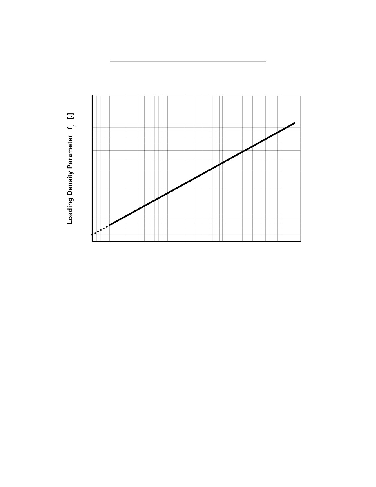
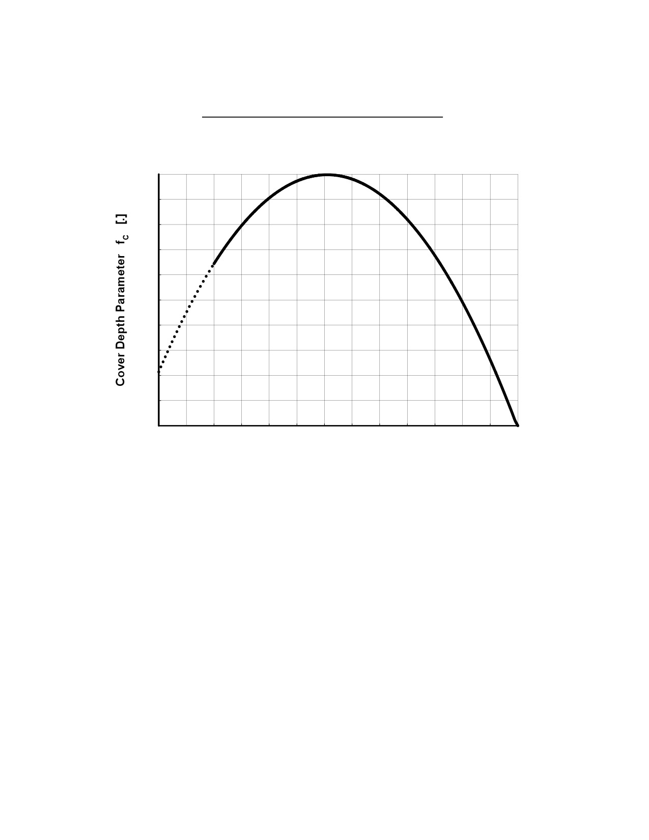
The loading density parameter, fγ can be taken from the graph in
Figure 3-XIX and the cover depth parameter, fc , from Figure 3-XX.
Both values can also be calculated with the corresponding formula
in Figures
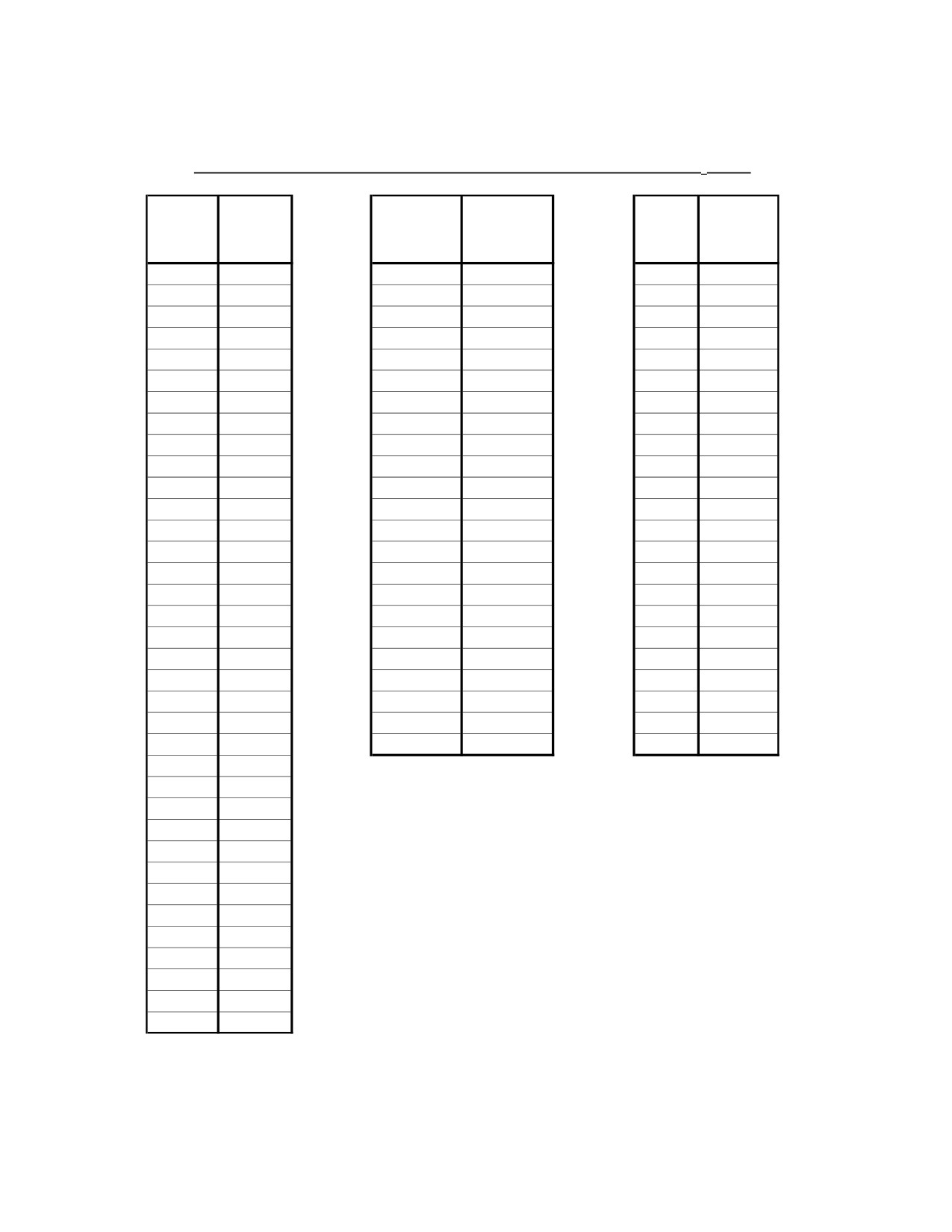
3-XIX and 3-XX. To simplify the calculation process
Figure 3-XXI contains tables for Q1/3, fγ and fc over a wide range of
commonly required values.
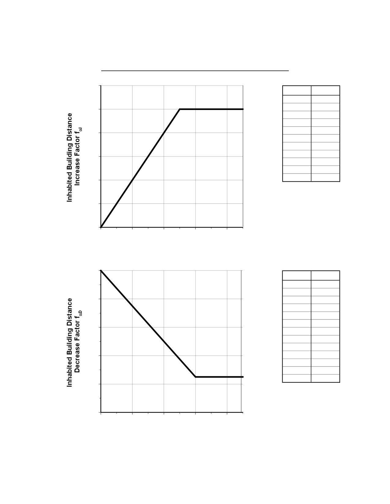
The loading density parameter, fα and the Inhabited Building
Distance increase with an increase in loading density. The cover
depth parameter (fc) is maximum at a scaled depth of C/Q1/3 =
approx. 0.5. The biggest crater is formed and the largest amount of
crater debris is thrown out into the surroundings at this scaled
depth, so the largest IBD results. As the scaled overburden
thickness increases above or decreases below the optimum depth
of burst, both the cover depth parameter (fc) and Inhabited Building
Distance decreases.
The influence of the slope angle of the overburden on the Inhabited
Building Distance is shown in Figure 3-XXII.
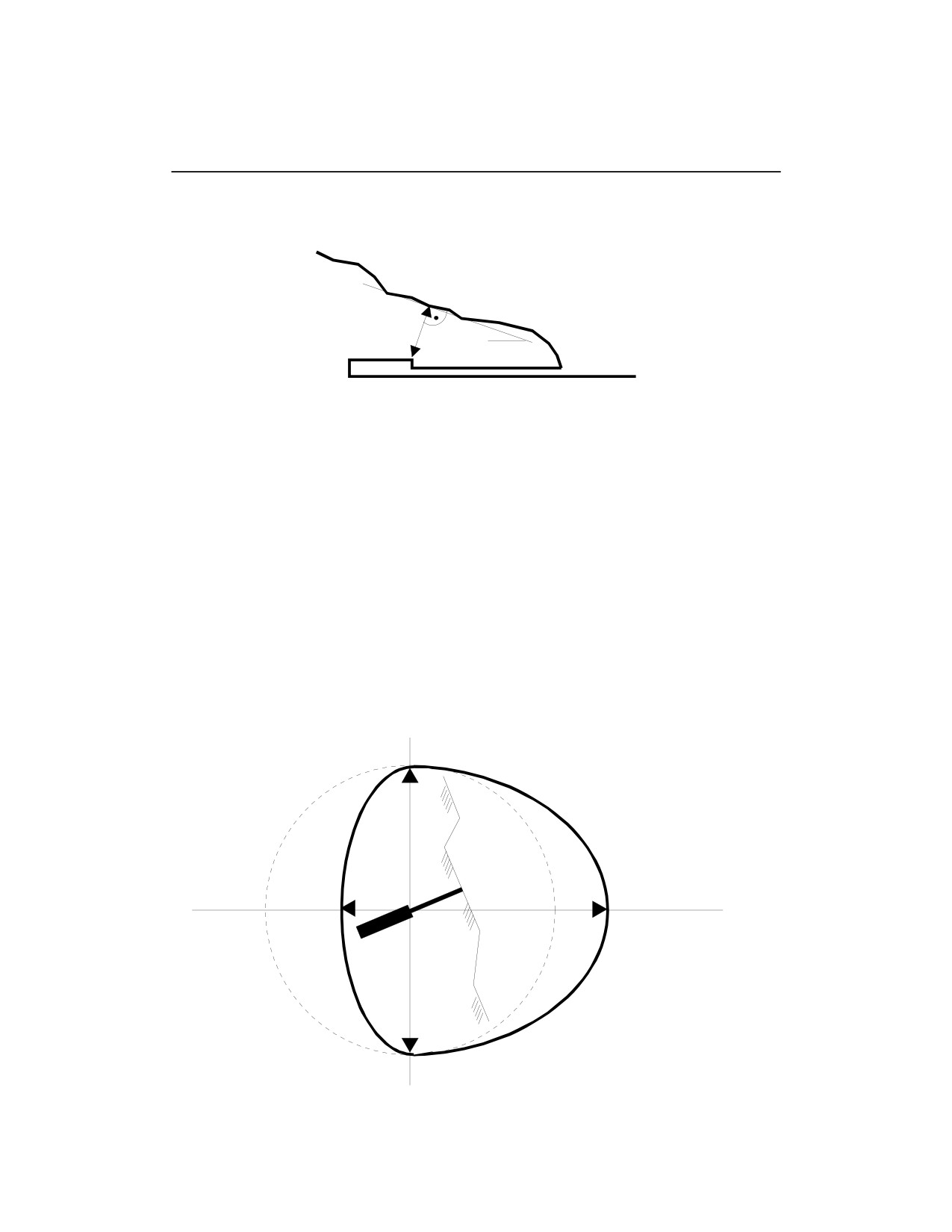
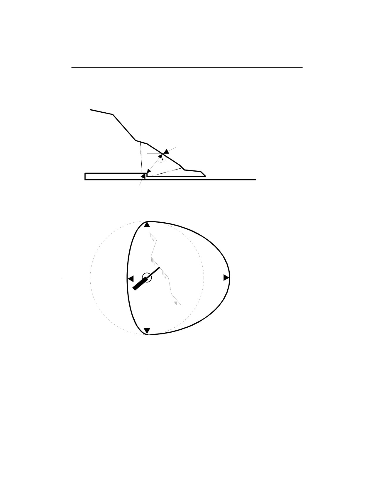
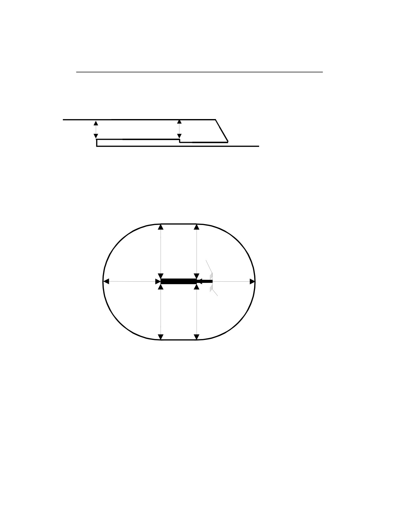
Figures 3-XXIV and 3-XXV show in general how the final IBD
contour line has to be established and the consideration of the
overburden slope angle parameter fα
Figure
3-XXIII, which is an example, illustrates a quantitative
determination of IBD for crater debris.
c)
IBD should be increased by 15% for an installation built in soft rock.
d)
Additional information:
The Inhabited Building Distance (IBD) has to be measured as a
horizontal distance from the crater-centre at the bottom of the crater
(CCB), at the level of the installation (Figure 3-XXIV).
The slope angle α shall be established in the area where the crater-
centre at the surface (CCS) has to be expected.
An average value for the slope angle α over the whole crater area
shall be taken in case the surface is not plain in this area.
The increase (fαI) and the decrease (fαD) factor must be applied to
the IBD in direction of the line with the largest gradient intersecting
the centre of the crater
(CCB). This line does not necessarily
coincide with the axis of the adit tunnel.
NATO/PFP UNCLASSIFIED
-III-3-39-
Change 3

NATO/PFP UNCLASSIFIED
AASTP-1
(Edition 1)
No increase or decrease factors need applied to the side of the
crater.
The shape of the IBD contour is elliptical.
In cases where more than one crater-centre is possible (e.g. in
cases of a flat rock overburden surface), the IBD has to be applied
from each possible crater-centre. The IBD contour shall be the
outer connection of the single lines (Figure 3-XXV).
e)
Limitations:
This crater debris throw model is based on an empirical evaluation
of the available data and engineering judgment of a comparatively
small number of tests and accidents. The overall accuracy is
therefore limited to the range of the investigated cases. Thus, the
crater debris throw model may be used only within the following
boundaries:
quantity of explosives NEQ =
1 t - 2000 t
chamber loading density γ
=
1 kg/m3 - 300 kg/m3
scaled cover depth C/Q1/3 >
0.1 m/kg1/3
In case of parameters exceeding these values it is appropriate to
take special care when applying the model.
NATO/PFP UNCLASSIFIED
-III-3-40-
Change 3
NATO/PFP UNCLASSIFIED
AASTP-1
(Edition 1)
Figure 3-XIX:
Loading Density Parameter fγ
1
0.1
1
10
100
1000
Loading Density γ = Q / Vc
[kg/m3]
f
= (γ / 1600) 0.35
γ
Q
= Weight of Explosives, NEQ
[kg]
VC
= Storage Chamber Volume
[m3]
NATO/PFP UNCLASSIFIED
-III-3-41-
Change 3
NATO/PFP UNCLASSIFIED
AASTP-1
(Edition 1)
Figure 3-XX:
Cover Depth Parameter fc
1.0
0.9
0.8
0.7
0.6
0.5
0.4
0.3
0.2
0.1
0.0
-0.1
0.0
0.1
0.2
0.3
0.4
0.5
0.6
0.7
0.8
0.9
1.0
1.1
1.2
Scaled Cover Depth C / Q 1/3
[m/kg1/3]
fC = 0.45 + 2.15 ∗ x - 2.11 ∗ x2
; x = C / Q 1/3
C = Overburden, Cover
[m]
Q = Weight of Explosives, NEQ
[kg]
NATO/PFP UNCLASSIFIED
-III-3-42-
Change 3
NATO/PFP UNCLASSIFIED
AASTP-1
(Edition 1)
Figure 3-XXI :
Auxilliary Tables for the Calculation of Q1/3, Fc and fϒ
Scaled
Loading
Q
Q1/3
Cover Depth
fC
Density
fγ
[kg]
[kg1/3]
[m/kg1/3]
[.]
[kg/m³]
[.]
1'000
10.0
0.10
0.64
1
0.08
1'500
11.4
0.15
0.73
3
0.11
2'000
12.6
0.20
0.80
5
0.13
2'500
13.6
0.25
0.86
10
0.17
3'000
14.4
0.30
0.91
15
0.20
4'000
15.9
0.35
0.94
20
0.22
5'000
17.1
0.40
0.97
25
0.23
6'000
18.2
0.45
0.99
30
0.25
7'000
19.1
0.50
1.00
40
0.27
8'000
20.0
0.55
0.99
50
0.30
0.60
0.98
60
0.32
10'000
21.5
0.65
0.96
70
0.33
15'000
24.7
0.70
0.92
80
0.35
20'000
27.1
0.75
0.88
90
0.37
25'000
29.2
0.80
0.82
100
0.38
30'000
31.1
0.85
0.75
120
0.40
40'000
34.2
0.90
0.68
140
0.43
50'000
36.8
0.95
0.59
160
0.45
60'000
39.1
1.00
0.49
180
0.47
70'000
41.2
1.05
0.38
200
0.48
80'000
43.1
1.10
0.26
220
0.50
1.15
0.13
250
0.52
100'000
46.4
1.20
0.00
300
0.56
150'000
53.1
200'000
58.5
250'000
63.0
300'000
66.9
400'000
73.7
Q = Weight of Explosives, NEQ
500'000
79.4
600'000
84.3
700'000
88.8
800'000
92.8
1'000'000
100.0
1'500'000
114.5
2'000'000
126.0
NATO/PFP UNCLASSIFIED
-III-3-43-
Change 3
NATO/PFP UNCLASSIFIED
AASTP-1
(Edition 1)
Figure 3-XXII:
Overburden Slope Angle Parameter fα
1.6
α
f α I
0.0
1.00
constant
2.5
1.05
1.5
5.0
1.10
7.5
1.15
fα I
= 1 +
0.02 ∗ α
10.0
1.20
1.4
12.5
1.25
15.0
1.30
17.5
1.35
1.3
20.0
1.40
22.5
1.45
> 25
1.50
1.2
1.1
1.0
0
10
20
30
40
Slope Angle α
[°]
1.0
α
f
α D
0.0
1.00
2.5
0.94
0.8
5.0
0.88
7.5
0.81
10.0
0.75
12.5
0.69
0.6
15.0
0.63
17.5
0.56
20.0
0.50
0.4
22.5
0.44
25.0
0.38
f
= 1 - 0.025 ∗ α
α D
constant
27.5
0.31
> 30
0.25
0.2
0.0
0
10
20
30
40
Slope Angle α
[°]
NATO/PFP UNCLASSIFIED
-III-3-44-
Change 3
NATO/PFP UNCLASSIFIED
AASTP-1
(Edition 1)
Figure 3-XXIII:
How to Calculate IBD's for Crater Debris Throw - Example
Given:
C
α
VC
VC
= 5000 m3
NEQ = 200'000 kg = Q
C
= 50 m
a
= 20 °
Solution: Q1/3 (from Figure XII)
= 58.5 kg1/3
Loading Density
= Q / VC
= 200'000 / 5000
= 40 kg/m3
Scaled Cover Depth
= C / Q1/3
= 50 / 58.5
= 0.85 m/kg1/3
Loading Density Parameter (from Figure X or XII)
fγ
= 0.27
Cover Depth Parameter (from Figure XI or XII)
fC
= 0.75
IBDF
= 38.7 ∗ Q1/3 ∗ fγ * fC
= 38.7 ∗ 58.5 ∗ 0.27 * 0.75
= 458 m
IBD Increase Factor (from Figure XIII)
fαI
= 1.4
IBD Decrease Factor (from Figure XIII)
fαD
= 0.5
IBD
= IBDF ∗ fαD
Line of Largest Gradient
229 m = 458 m ∗ 0.5
IBD
= IBDF ∗ fαI
641 m = 458 m ∗ 1.4
Shape: Elliptical
IBD = IBDF = 458 m
NATO/PFP UNCLASSIFIED
-III-3-45-
Change 3
NATO/PFP UNCLASSIFIED
AASTP-1
(Edition 1)
Figure 3-XXIV:
How to Establish Inhabited Building Distance Contrours
Cross Section of Installation
CCS
α
C
CCB
Inhabited Building Distance Contour
(ground-plan)
IBD = IBD
IBD = IBDF ∗ fαI
F ∗ fαD
CCB
Line of Largest Gradient
Shape: Elliptical
IBD = IBDF
α
= Slope Angle of Overburden
C
= Cover / Overburden
CCS
= Crater-Center-Surface
CCB
= Crater-Center-Bottom
IBDF
= Inhabited Building Distance
for Flat Terrain / Overburden
= Inhabited Building Distance Increase Factor
fαI
fαD
= Inhabited Building Distance Decrease Factor
NATO/PFP UNCLASSIFIED
-III-3-46-
Change 3
NATO/PFP UNCLASSIFIED
AASTP-1
(Edition 1)
Figure 3-XXV:
How to Establish Inhabited Building Distance Contrours
Cross Section of Installation
Flat Overburden
C
C
Inhabited Building Distance Contour
(ground-plan)
IBD = IBDF
IBD = IBDF
IBD = IBDF
IBD = IBDF
C
= Cover / Overburden
IBDF
= Inhabited Building Distance
for Flat Terrain / Overburden
NATO/PFP UNCLASSIFIED
-III-3-47-
Change 3

NATO/PFP UNCLASSIFIED
AASTP-1
(Edition 1)
3.3.4.3 Ground Shock
1
Introduction
The prediction of ground shock and the derivation of its quantity-distances require
careful consideration of the all factors affecting ground shock propagation and the
ground shock parameters.
1.1
Factors Affecting Ground Shock Effects
Ground shock is highly site-dependent and is affected by the following factors:
a.
Geological structure and rock mass properties
b.
Explosives charge weight and scaled range
c.
Chamber loading density
d.
Charge distribution and chamber volume
1.2
Geological Classification
The geological classification presented in Table 1-I should be used for the prediction
of the ground shock parameters. If the rock type is not clear, the classification should
be based on wave propagation properties rather than on strength. Important rock
mass properties affecting wave propagation include bulk density, seismic wave
velocity, and joints and their orientation.
1.3
Geology of Site
The geology of a site is further classified into the following categories:
Single medium - where the Potential Explosion Site (PES) and Exposed Site
(ES) are in the same rock mass.
Mixed media - where the bedrock is overlain by a soil layer of a significant
thickness (typically with a soil-to-rock thickness ratio of 0.2), which affects
ground shock propagation and the frequency content of the ground shock
wave reaching the structure, and PES is in rock where the storage chambers
are sited and ES in a soil overburden on which buildings are found.
For cases where the soil cover is less than 0.05 of the transmission distance
or less than 5 m, the site geology may be classified as single medium.
1.4
Ground Shock Parameters
The prediction of ground shock must be done with a view for the assessment
of structural response. A complete definition of the ground shock wave is the
response spectra, which can be generated either empirically or numerically.
NATO/PFP UNCLASSIFIED
-III-3-48-
Change 3

NATO/PFP UNCLASSIFIED
AASTP-1
(Edition 1)
For assessment of structural response, the most important parameters for
ground shock are the magnitude and the frequency content. The magnitude is
often expressed by the Peak Particle Velocity (PPV) while the frequency
content can be represented by the Principal Frequency (PF). If possible,
calculations should be made for both the vertical and horizontal components
of the ground shock wave.
2
Prediction Equations for PPV and PF
The Peak Particle Velocity
(PPV) and Principal Frequency (PF) equations can
generally be described as follows, respectively:
−m
⎛
R
⎞
PPV
=
A⎜
⎟
⎜
1/3
⎟
⎝Q
⎠
−n
⎛
R
⎞
PF
=
B⎜
⎟
⎜
1/
3 ⎟
Q
⎝
⎠
where
PPV
= Peak Particle Velocity
[m/s]
PF
= Principal Frequency
[Hz]
R
= Radial distance measured from the chamber wall along a line drawn
from the chamber centre to the point of interest on the ground surface
[m]
Q
= Net Explosives Quantity
[kg]
A and B are initial values at scaled range, R/Q1/3 = 1.0 m/kg1/3; and
m and n are the attenuation coefficients.
Summary tables of the initial values and attenuation coefficients for the Peak Particle
Velocity (PPV) and Principal Frequency (PF) prediction equations are presented in
Table 1-II and Table 1-III respectively.
The results cover charge weights up to 500 tonnes, chambers of length ranging from
45 to 120 m with maximum volume of 50,000 m3, and span to length ratio between
1:2 and 1:4. The loading densities considered range up to 50 kg/m3 with rock cover
or equivalent cover of about 1.0Q1/3 m.
3
Frequency-based Ground Shock IBD for Reinforced Concrete (RC) Structures
3.1
Response of Structures due to Ground Shock
NATO/PFP UNCLASSIFIED
-III-3-49-
Change 3

NATO/PFP UNCLASSIFIED
AASTP-1
(Edition 1)
The damage of a building due to ground shock can be characterised by the reduction
in natural frequency of the structural system. This can be represented by a building
damage index (DI), which can be calculated using the following equation:
2
f
i
BDI =
1
−
2
f
p
where
f
= Initial natural frequency
[Hz]
i
f
p
= Post-event natural frequency of structure
[Hz]
3.2
Classification of Building Damage
Building damage due to ground shock can be classified into the following categories
given in Table 2-I.
3.3
Prediction of Building Damage Index
The building damage index (DI) of a typical reinforced concrete structure up to ten
storeys, with span up to 5 m and inter-storey height up to 3m, can be obtained for a
given Peak Particle Velocity (PPV) and Principle Frequency (PF).
The equations for the prediction of PPV and PF can be found in Section 2. If other
methods are used to predict the PPV in the horizontal and vertical directions, the
resultant PPV should be used, and can be calculated from the following equation:
2
2
PPV =
PPV
x
+ PPV
y
where
PPVx = maximum peak particle velocity in the horizontal direction
[m/s]
PPVy
= maximum peak particle velocity in the vertical direction
[m/s]
3.4
Criteria for Ground Shock IBD
The recommended building damage index (DI) to adopt is 0.4. At this value, the
building is expected to suffer only repairable minor damage, where small cracks
occur in the concrete, but the reinforcement will remain in the elastic range. The
overall stiffness will be reduced by 20 - 40%. Collapse of buildings is not expected
and fatality is unlikely. If a higher damage index were to be adopted, the ground
shock IBD equations in Section 3.5 would have to be adjusted accordingly. Studies
related lethality rates and the associated damage index could be used to guide the
selection of the acceptable damage index.
NATO/PFP UNCLASSIFIED
-III-3-50-
Change 3

NATO/PFP UNCLASSIFIED
AASTP-1
(Edition 1)
3.5
Ground Shock IBD for Reinforced Concrete (RC) Structures
The response and damage of buildings are primarily governed by the magnitude
(PPV) and frequency content (PF) of the ground shock. Based on an acceptable
building damage index of 0.4 as given in the previous section, the allowable PPV for
reinforced concrete structures will be given as:
PPV < 0.4 m/s
for
10 Hz < PF < 30 Hz
PPV < 0.0825 PF0.46 m/s
for
30 Hz < PF < 100 Hz
PPV < 0.7 m/s
for
100 Hz < PF
The IBD for the siting of reinforced concrete structures is:
1
1
−
m
3
IBD = (
)
*(Q
)
for 10 Hz < PF < 30 Hz
A
0.46
1
1
0.0825B
(−m+0.46n)
3
IBD = (
)
*(Q
)
for 30 Hz < PF < 100 Hz
A
1
1
−
m
3
IBD = (
)
*(Q
)
for 100 Hz < PF
A
Where IBD is in metres, measured directly from the chamber wall, and A, B, m and n
are constants given in Table 1-II and 1-III.
Since the PF is also a function of the distance, the user should check the PF and
ensure that the correct IBD equation from the above is used. Iterative calculations
may be required to solve for the ground shock IBD.
Example #1:
Given: Q = 125,000kg
Loading density = 20kg/m3 Span-length ratio = 1:2
Geology: Single Medium, Good Rock
Equivalent cover thickness = 1.0 Q1/3
Solution: From Table 1-II and 1-III, A = 1.35, m = 1.23, B = 72, n = 0.84
−
1
1
−
1
m
3
1.23
IBD = (
)
*(Q
) = (
)
*(125,0003)1
= 134 metres
A
1.35
R
−n
134
−0.84
Check PF = B(
1
/
3
)
= 72(
1/3
)
= 31 Hz > 30 Hz => Not OK!
Q
125,000
1
1
1
0.0825B
0.46
(−m+0.46n)
3
0.0825*72
0.46
(−1.23+0.46*0.84
)
IBD = (
)
*(Q
)
=(
)
*(125,0003)1
= 133 metres
A
1.35
R
−n
133
−0.84
Check PF = B(
1
/
3
)
= 72(
1/3
)
= 32 Hz > 30 Hz and < 100Hz => Ok!
Q
125,000
Example #2:
Given: Q = 125,000kg
Loading density = 20kg/m3 Span-length ratio = 1:2
Geology: Mixed media with Good Rock Soil to rock cover ratio = 0.2
NATO/PFP UNCLASSIFIED
-III-3-51-
Change 3