PowerWorld Simulator version 11. Manual - page 18
PowerWorld Simulator Add-on Tools
OPF Options : Solution Results
The OPF Dialog, Solution Results page displays general results from the last OPF solution. The display contains the
following fields, none of which can be directly changed:
General Results
Solution Start Time, Solution End Time
The starting time and ending time of the OPF solution algorithm.
Total Solution Time, Last Solution Status
Time and status of the last OPF solution.
Number of LP Iterations
Total number of LP iterations used during the last OPF solution. The maximum number of iterations are specified in
the Maximum Number of Iterations field of the General Options page.
Initial Cost Function Value
Initial value of the OPF cost function. During the OPF the solution algorithm seeks to minimize the cost function,
subject to the equality and inequality constraints.
Final Cost Function Value
Final value of the OPF cost function.
Final Slack Cost Value
The slack cost value is an artificial cost that is only non-zero when there are one or more unenforceable constraints.
Final Total Cost Value
The addition of the final cost function value and the final slack cost value.
Number of Buses in OPF
This field contains the total number of buses that are in areas or super areas that are on OPF control. Thus this
field need not be equal to the total number of buses in the case. Marginal costs are only calculated for buses in
OPF controlled areas or super areas.
Highest Bus Marginal Cost, Lowest Bus Marginal Cost, Average Bus Marginal Cost
Highest, lowest and average marginal cost for the buses that are in OPF controlled areas or super areas.
Bus MC Standard Deviation
The standard deviation of the Bus Marginal Cost.
Line MVA Constraints
The Line MVA Constraints fields present results associated with the enforcement of the line MVA constraints.
Number of Initial Violations, MVA Sum of Initial Violations
Total number of lines that initially exceeded their MVA limits and were eligible for enforcement by the OPF. For
these lines only, the MVA Sum of Initial Violations field contains sum of the absolute values of the line's actual
MVA flow minus the line's MVA limit.
Number of Binding Lines
Total number of lines that are constrained to their limit value.
Highest Line MVA Marginal Cost
The highest Marginal Cost for an MVA change on a line.
Number of Unenforceable Violations
Total number of lines whose MVA flows can not be enforced by the OPF using the available controls.
MVA Sum of Unenforceable Violations
For all the unenforceable lines, this field contains the sum of the absolute values of the line's actual MVA flow minus
the line's MVA limit.
Interface MW Constraints
The Interface MW Constraints field present results associated with the enforcement of the interface MW constraints.
Number of Initial Violations, MW Sum of Initial Violations
677
Total number of interfaces that initially exceeded their MW limits and were eligible for enforcement by the OPF. For
these interfaces only, the MW Sum of Initial Violations field contains sum of the absolute values of the interface's
actual MW flow minus the interface's MW limit.
Number of Binding Interfaces
Total number of interfaces that are constrained to their limit value.
Highest Interface MW Marginal Cost
The highest Marginal Cost for an MVA change on an interface.
Number of Unenforceable Violations
Total number of interfaces whose MW flows can not be enforced by the OPF using the available controls.
MW Sum of Unenforceable Violations
For all the unenforceable interfaces, this field contains the sum of the absolute values of the interface's actual MW
flow minus the interface's MW limit.
Area and Superarea Constraints
Unenforceable Area Constraints
Number of unenforceable area constraints.
Unenforceable Superarea Constraints
Number of unenforceable superarea constraints.
678
PowerWorld Simulator Add-on Tools
OPF Options: All LP Variables
The OPF Dialog, All LP Basic Variables page displays the basic and non-basic variables associated with the final LP
solution. This page is usually only of interest to users interested in the specifics of the LP solution. Right click any
where in the display to copy a portion or all of the display to the Window's clipboard, or to print the results.
The display lists each of the LP variables, showing the following fields for each:
ID
Variable identifier.
Original Value
The initial value of the LP variable before SCOPF optimization.
Value
The final value of the LP variable after OPF optimization.
Delta Value
The difference between the original value field and the value field.
Basic Var
Shows the index of the basic variables in the LP basis. If the value is zero, the variable is non-basic.
NonBasicVar
Shows the index of the non-basic variable. If the value is zero, the variable is basic.
Cost(Down)
The cost associated with decreasing the LP variable. The field will show if the variable is at its max or min limit.
Cost(Up)
The cost associated with increasing the LP variable. The field will show if the variable is at its max or min limit.
Down Range
The available range to decrease the basic variable before a new constraint is hit under a contingency condition.
Up Range
The available range to increase the basic variable before a new constraint is hit under a contingency condition.
Reduced Cost Up
The cost reduction that would be experimented if a LP variable increases. If a constraint is at the limit, the field
shows the change in cost of constraint enforcement.
Reduced Cost Down
The cost reduction that would be experimented if a LP variable decreases. If a constraint is at the limit, the field
shows the change in cost of constraint enforcement.
At Breakpoint?
Yes, if the LP variable is at a break point.
679
OPF Options: LP Basic Variables
The OPF Dialog, LP Basic Variables page displays the basic variables associated with the final LP solution. This page
is usually only of interest to users interested in the specifics of the LP solution. Right click any where in the display to
copy a portion or all of the display to the Window's clipboard, or to print the results.
The display lists each of the basic variables, showing the following fields for each:
ID
Basic variable identifier.
Original Value
The initial value of the basic LP variable before the OPF optimization.
Value
The final value of the basic LP variable after the OPF optimization.
Delta Value
The difference between the original value field and the value of the basic variable.
Basic Var
Shows the indices of the basic variables in the LP basis.
Cost(Down)
The cost associated with decreasing the basic variable.
Cost(Up)
The cost associated with increasing the basic variable.
Down Range
The available range to decrease the basic variable before a new constraint is hit under a contingency condition.
Up Range
The available range to increase the basic variable before a new constraint is hit under a contingency condition.
680
PowerWorld Simulator Add-on Tools
OPF Options: LP Basis Matrix
The OPF Dialog, LP Basis Matrix page displays the basis matrix associated with the final LP solution. This page is
usually only of interest to users interested in knowing the specifics of the LP solution. Knowing the basis matrix can be
helpful in figuring out why a particular power system is exhibiting a particular behavior. The rows of the basis matrix
are the binding constraints, while the columns of the basis matrix are the basic variables. The entries in the basis
matrix then give the sensitivity of each constraint to each of the basic variables. The width of the columns in the matrix
can also be adjusted using the Column Widths field. Finally, right-click somewhere in the matrix to copy the matrix to
the Window's clipboard or to print the matrix.
681
OPF Options: Bus MW Marginal Price Details
The Bus MW Marginal Price Details page displays a grid containing the MW marginal prices computed for an OPF
solution. If no OPF solution has been run, the values will all be zero. The grid used for displaying the information is a
Case Information Display, which can be modified, sorted, printed, etc., as described in the discussion of Case
Information Displays.
682
PowerWorld Simulator Add-on Tools
OPF Options: Bus MVAR Marginal Price Details
The Bus MVAR Marginal Price Details page displays a grid containing the MVAR marginal prices computed for an
OPF solution. If no OPF solution has been run, or if the option to compute MV AR marginal prices has not been
selected, the values will all be zero. The grid used for displaying the information is a Case Information Display, which
can be modified, sorted, printed, etc., as described in the discussion of Case Information Displays.
683
OPF Options: Bus Marginal Controls
This display shows the sensitivities of the controls with respect to the cost at each bus. A change in a system control
will have the indicated effect in the marginal cost at the system buses. Vice-versa, the marginal cost at a bus is
affected by changes in the value of the basic variables.
684
PowerWorld Simulator Add-on Tools
OPF Options: Inverse of LP Basis
The OPF Dialog, LP Basis Matrix page displays the inverse of the basis matrix. The width of the columns in the matrix
can also be adjusted using the Column Widths field. Finally, right-click somewhere in the matrix to copy the matrix to
the Window's clipboard or to print the matrix.
685
OPF Records
OPF Area Records
Displays OPF specific information about each area record in the case. To show this display select LP OPF, OPF Area
Records . The OPF Area Records Display is a class of Case Information Display and therefore can be used in a
manner consistent with the other case information displays. Specific formatting options are available from the local
menu, which can be accessed by right-clicking on any field in the display. The columns can also be sorted by right-
clicking on the heading of the field.
By default the display contains the following fields:
Number, Name
Area’s number, between 1 and 999, and its alphanumeric identifier, eight characters maximum.
AGC Status
Area's automatic generation control status. This is the same field shown on the Area Records Display. The field
indicates whether or not the area's generation is changing automatically to control the area interchange.
To be included in the OPF, this field MUST be "OPF". The generation costs for areas that are on "OPF" control are
included in the OPF objective function; otherwise they are not. Note that if the area is part of a super area that is on
AGC control, this field value is ignored.
Double-click on the field to toggle its value.
XF Phase
Specifies whether phase shifting transformers in the area are available as controls. If "Yes" then all transformers in
the area which have their Automatic Control Active are available for control; the Automatic Control status for a
transformer is set on the Line/Transformer Dialog. If "No" then no transformers in the area are available for control.
Branch MVA
Specifies whether or not the MVA limits should be enforced for transmission lines and transformers that have at
least one terminal in this area. For a transmission line or transformer to be included Line/Transformer constraints
must not be disabled on the OPF Options Dialog, and the individual line/transformer must be enabled for
enforcement on the OPF Line/Transformer MVA Constraints display.
Interface MW
Specifies whether or not the MW limits should be enforced for interfaces that have at least one element in this area.
For an interface to be included Interface constraints must not be disabled on the OPF Options Dialog, and the
individual interfaces must be enabled for enforcement on the OPF Interface MW Constraints display.
Load MW Dispatch
Specifies whether or not the MW load demand in an area should be included as available for re-dispatch during an
OPF solution. In order for loads to be included in OPF re-dispatch, each individual load within the area must be
available for control, and have either a fixed cost benefit or a piecewise-linear cost benefit curve provided.
Include Marg. Losses
Specifies whether or not marginal losses should be included for the area during the OPF solution.
MW Marg. Cost Ave
For an OPF solved case this field shows the average of the bus MW marginal costs for all the buses in the area. If
there is no congestion then all of the marginal costs should be equal.
MW Marg. Cost St.Dev., Min., Max.
For an OPF solved case these fields show the standard deviation of the bus MW marginal costs for all the buses in
the area, the minimum and the maximum bus MW marginal costs.
Report Limits
Specifies whether or not the kV limits should be reported.
Report Min kV, Report Max kV
Specifies the values for minimum and maximum kV levels to report. Defaults are 0 and 9999.
686
PowerWorld Simulator Add-on Tools
OPF Bus Records
Displays OPF specific information about each bus record with a valid area/zone/owner filter. To show this display
select LP OPF, OPF Bus Records. The OPF Bus Records Display is a class of Case Information Display and
therefore can be used in a manner consistent with the other case information displays. Specific formatting options are
available from the local menu, which can be accessed by right-clicking on any field in the display. The columns can
also be sorted by right-clicking on the heading of the field.
By default the display contains the following fields
Number, Name
Bus’s number, between 1 and 99,999, and its alphanumeric identifier, eight characters maximum.
Area Name
Name of the bus's area.
MW Marg. Cost
Marginal change in the objective function for a one MW change in the real power load at the bus.
MVR Marg. Cost
Marginal change in the objective function for a one Mvar change in the reactive load at the bus.
Volt Marg. Cost
Marginal change in the objective function for a 0.01 per unit change in the voltage setpoint for the bus. This field is
only valid at bus’s whose terminal voltage is controlled by one or more generators.
Note from the developers - this field is still under construction - do not use it yet.
687
OPF Generator Records
Displays OPF specific information about each generator record with a valid area/zone/owner filter. To show this
display select LP OPF > OPF Generator Records . The OPF Generator Records Display is a class of Case
Information Display and therefore can be used in a manner consistent with the other case information displays.
Specific formatting options are available from the local menu, which can be accessed by right-clicking on any field in
the display. The columns can also be sorted by right-clicking on the heading of the field.
By default the display contains the following fields
Number, Name
Number and name of the bus to which the generator is attached. The display's local menu offers you the
opportunity to view the Quick Power Flow List and the Bus View Display for this bus. You can also use the local
men to view the generator's dialog.
ID
Alphanumeric ID used to distinguish multiple generators at the same bus.
Area Name of Gen
Name of the generator's area.
AGC
Designates whether the generator's real power output is governed by automatic generation control (AGC). If the
AGC field is set to Yes the generator is on AGC in the standard power flow. When a generator is on AGC its real
power output is varied automatically, provided the generator is part of an area or super area that is also on
automatic control.
In Simulator OPF the default operating mode is that only generators on AGC control are eligible to be OPF controls.
In addition, the generator's area or super area must have AGC Status of "OPF". However in rare instances you
may wish to always make a generator available for control or never make the generator available for control. This
value is specified using OPF MW Control field.
Fast Start
Designates whether the generator is available as a Fast Start generator during the OPF solution process. Fast start
generators are another type of control available to the Optimal Power Flow solution routine. The OPF routine can
determine if a generator labeled as a fast start generator would be beneficial in reducing the overall system costs of
generation dispatch. If a fast start generator is off-line, but could reduce the cost of the system, then the OPF
routine will turn on the generator, and increase the generator's dispatch towards optimizing the system generating
cost. Conversely, if a fast start generator is on-line, and the OPF routine determines that reducing the generator's
output to 0 would reduce the total generation cost, then the OPF routine will shut off the generator.
Generally speaking, the fast start options should only be used with units with zero Minimum MW limits. Hence it is
really aimed at hydro units, or small units which do not need a non-zero minimum MW output for valid operation.
This requirement is needed because changing a unit's status is only valid in the OPF routine if it is determined that
the unit should dispatch 0 MW to optimize the generating costs of the system.
OPF MW Control
Designates whether the generator's real power output should be included as a control variable in the OPF. This
field, which can be toggled, has three possible values:
· "If AGCable" - Generator's control availability depends upon its AGC status.
· "Yes" - Generator is available as a control, regardless of its AGC status.
· "No" - Generator is NOT available as a control, regardless of its AGC status.
Note: in order to be a control the generator must also be in an area or super area on "OPF" control.
Gen MW
The real power output of the generator.
Cost Shift $/MWh, Cost Multiplier
The cost shift and cost multiplier allow you to easily apply a shift to the cost function for the purpose of assessing
how variations in bids impact profit. The cost function is affected based on the following equation:
(Original Cost Function + Cost Shift) * Cost Multiplier
Cost $/Hr
The total cost of the generator, including the impact of the cost shift and cost multiplier.
MW Marg. Cost
688
PowerWorld Simulator Add-on Tools
Tells the marginal cost, in $ / MWhr, to supply one additional MW of load at this bus. If a generator is available as a
control and is not at either its minimum or maximum limit or a cost model breakpoint, then the MW Marg. Cost field
will be identical to the generator's current marginal cost. However the usual case is for the generator to be at either
a limit or a cost model breakpoint so the usual situation is that the MW Marg. Cost field values IS NOT equal to the
generator's marginal cost.
IC for OPF
Incremental cost of the generator at its current operating point.
Initial MW
The initial real power output of the generator at the beginning of the OPF solution. You can reset the case back to
these values by selecting the LP OPF, Restore Previous Control Settings menu item. This menu item is only
available following a successful OPF solution.
Initial Cost
The initial generator cost at the beginning of the OPF solution.
Delta MW
Change in the generator's real power output as a result of the OPF.
Delta Cost
Change in the generator's cost as a result of the OPF.
Min MW, Max MW
Minimum and maximum real power output of the generator.
Cost Model
The current cost model being used for the generator. The field value is either "Cubic", indicating that the
generator's operating costs are being modeled using a cubic cost function, or "Piecewise Linear", indicating the
operating costs are being modeled using a piecewise linear cost function. Toggle the field to change the model.
Note that a generator may simultaneously have a cubic model and a piecewise linear model.
Because the OPF uses a linear programming approach, the generator's operating costs are ALWAYS modeled
using the piecewise linear model. Generators with an existing cubic cost model are either 1) ignored as OPF
controls, or 2) have a piecewise linear cost model automatically created from the cubic model, depending upon the
values specified on the OPF Options dialog.
# Cost Curve Points
Shows the number of segments in the piecewise linear model. If no piecewise linear model exists then this field is
zero; the generator's costs are being modeled using the cubic function. For such generators you can automatically
setup a piecewise linear model simply by entering a non-zero value for the number of points. A piecewise linear
model is created that matches as closely as possible the existing cubic model.
Fuel Type
Specifies the fuel type of the generator, if it is known; double-click to toggle through the options. Options are
Unknown, Coal, Gas, Hydro, Hydro Pumped, Nuclear, Petroleum, Solar, Wind, and Other.
Profit $/hr
Shows the profit of the generator. Profit is calculated using this equation:
Profit = (GenMW * MW Marg Cost ) - [ FuelCost*( IOA + IOB * GenMW + IOC * GenMW 2 + IOD * GenMW 3 ) ]
689
OPF Interface Records
Displays OPF specific information about the interface records in the case. To show select LP OPF > OPF Interface
Records. This display is actually a page of a display showing all the potential inequality constraints in the power
system. The top portion of the display repeats the fields shown on the Constraint Options page of the OPF Options
dialog.
To view the Interface records click on the Interfaces tab. This displays the interfaces page which is a class of Case
Information Display and therefore can be used in a manner consistent with the other case information displays.
Specific formatting options are available from the local menu, which can be accessed by right-clicking on any field in
the page. The columns can also be sorted by right-clicking on the heading of the field.
By default the Interface Records page contains the following fields:
Name
Name of the interface.
Monitor
Specifies whether or not the interface MW limit is enforced in the OPF solution.
Interface MW
The amount of MW flow on the interface.
MW Limit
The interface MW limit.
Percent
The amount of MW flow on the interface as a percentage of the limit.
Monitor Direction
The direction on the interface in which the flow is being monitored.
MW Marg. Cost $ / MWh
The marginal cost of enforcing the limit on the interface.
MW Unenforceable
This field will be set to YES if the interface limit is unenforceable in the OPF solution.
Constraint
This field will be set to YES if the interface limit is a constraint in the OPF solution.
690
PowerWorld Simulator Add-on Tools
OPF Nomogram Records
This list displays OPF specific information about the nomogram records in the case. To show the list, select LP OPF >
OPF Nomograms. This display is actually a page of a display showing all the potential inequality constraints in the
power system. The top portion of the display repeats the fields shown on the Constraint Options page of the OPF
Options dialog.
To view the nomogram records click on the Nomogram Interfaces tab. This displays the nomogram interfaces page
which is a class of Case Information Display and therefore can be used in a manner consistent with the other case
information displays. Specific formatting options are available from the local menu, which can be accessed by right-
clicking on any field in the page. The columns can also be sorted by right-clicking on the heading of the field.
By default the Interface Records page contains the following fields:
Nomo. Name
Name of the nomogram.
Nomo. Seg.
The segment of the nomogram. Each segment of the nomogram is treated as a separate constraint in the OPF,
and therefore is listed individually in the OPF nomogram table.
Monitor
This field will be set to YES if the nomogram segment is monitored during the OPF.
Interface MW
The total MW flow for the segment of the nomogram.
MW Limit
The segment MW limit.
Percent
The amount of MW flow on the segment as a percentage of the segment’s limit.
Monitor Direction
The direction on the segment in which the flow is being monitored.
MW Marg. Cost $ / MWh
The marginal cost of enforcing the limit on the segment.
MW Unenforceable
This field will be set to YES if the nomogram segment’s limit is unenforceable in the OPF solution.
Constraint
This field will be set to YES if the nomogram segment’s limit is a constraint in the OPF solution.
691
OPF Line/Transformer Records
Displays OPF specific information about the line and transformer records in the case. To show select LP OPF, OPF
Line/Transformer Records. This display is actually a page of a display showing all the potential inequality
constraints in the power system. The top portion of the display repeats the fields shown on the Constraint Options
page of the OPF Options dialog.
To view the Line and Transformer records click on the Line/Transformers tab. This displays the Line/Transformer
page which is a class of Case Information Display and therefore can be used in a manner consistent with the other
case information displays. Specific formatting options are available from the local menu, which can be accessed by
right-clicking on any field in the display. The columns can also be sorted by right-clicking on the heading of the field.
By default the display contains the following fields:
From Number, From Name, From Area Name
Number, Name, and Area Name of the From bus.
To Number, To Name, To Area Name
Number, Name, and Area Name of the To bus.
Circuit
Circuit identifier for the branch.
Monitor
Specifies whether or not the branch's MVA limit will be enforced in the OPF solution.
Max MVA
The maximum MVA flow on the branch. Value is determined based on the end of the branch with the higher MVA
flow.
% of MVA Limit (Max)
The maximum MVA flow as a percentage of the branch MVA limit. Value is determined based on the end of the
branch with the higher MVA flow.
Lim MVA
The MVA limit for the branch.
MVA Marg. Cost
The marginal cost of changing the MVA flow on the branch.
MVA Unenforceable
This field will be set to YES if the branch limit is unenforceable in the OPF solution.
Constraint
This field will be set to YES if the branch limit is a constraint in the OPF solution.
692
PowerWorld Simulator Add-on Tools
OPF Load Records
Displays OPF specific information about each load record with a valid area/zone/owner filter. To show this display
select LP OPF > OPF Load Records. The OPF Load Records Display is a class of Case Information Display and
therefore can be used in a manner consistent with the other case information displays. Specific formatting options are
available from the local menu, which can be accessed by right-clicking on any field in the display. The columns can
also be sorted by right-clicking on the heading of the field.
By default the display contains the following fields
Number, Name
Number and name of the bus to which the load is attached. The display's local menu offers you the opportunity to
view the Quick Power Flow List and the Bus View Display for this bus. You can also use the local menu to view the
generator's dialog.
ID
Alphanumeric ID used to distinguish multiple loads at the same bus.
Area Name of Load
Name of the load’s area.
AGC
Designates whether the load’s real power demand is governed by automatic generation control (AGC). If the AGC
field is set to Yes the load is on AGC in the standard power flow. When a load is on AGC its real power output is
varied automatically during an OPF or SCOPF solution ONLY, provided the load is part of an area or super area
that is also on OPF control. Loads will not be dispatched if the area is on some other form of AGC control.
In Simulator OPF the default operating mode is that only loads on AGC control are eligible to be OPF controls. In
addition, the load’s area or super area must have AGC Status of "OPF", and the area must have its Load MW
Dispatch set to YES.
MW
The real power output of the load.
Cost Shift $/MWh, Cost Multiplier
The cost shift and cost multiplier allow you to easily apply a shift to the cost function for the purpose of assessing
how variations in bids impact profit. The cost function is affected based on the following equation:
(Original Cost Function + Cost Shift) * Cost Multiplier
Hourly Benefit
The total benefit of the load, including the impact of the cost shift and cost multiplier.
MW Marg. Cost
Tells the marginal cost, in $ / MWhr, to reduce one additional MW of load at this bus. If a load is available as a
control and is not at either its minimum or maximum limit or a cost model breakpoint, then the MW Marg. Cost field
will be identical to the load’s current marginal cost. However the usual case is for the load to be at either a limit or a
cost model breakpoint so the usual situation is that the MW Marg. Cost field value IS NOT equal to the load’s
marginal cost.
Inc. Benefit
Incremental benefit of the load at it’s current operating point.
Initial MW
The initial real power demand of the generator at the beginning of the OPF solution. You can reset the case back to
these values by selecting the LP OPF > Restore Previous Control Settings menu item. This menu item is only
available following a successful OPF solution.
Initial Cost
The initial load cost at the beginning of the OPF solution.
Delta MW
Change in the load's real power output as a result of the OPF.
Delta Cost
Change in the load's cost as a result of the OPF.
Min MW, Max MW
Minimum and maximum real power demand of the load.
693
# of Benefit Curve Points
Shows the number of segments in the piecewise linear model. If no piecewise linear model exists then this field is
zero.
Profit $/hr
Shows the profit of the load.
694
PowerWorld Simulator Add-on Tools
OPF Super Area Records
Displays OPF specific information about each super area record in the case. To show this display select LP OPF,
OPF Super Area Records. The OPF Super Area Records Display is a class of Case Information Display and
therefore can be used in a manner consistent with the other case information displays. Specific formatting options are
available from the local menu, which can be accessed by right-clicking on any field in the display. The columns can
also be sorted by right-clicking on the heading of the field.
By default the display contains the following fields:
Super Area
Alpha-numeric identifier of the super area.
AGC Status
Super area's automatic generation control status. This is the same field shown on the Super Area Records display.
The field indicates whether or not the super area's generation is changing automatically to control the super area's
interchange.
The super area AGC Status field always overrides the AGC Status for the individual areas, except when it is set to
"Off AGC".
To be included in the OPF this field MUST be "OPF". In that case the generation costs for all the areas in the super
area are included in the OPF objective function. Otherwise they are only included if the super area AGC Status is
"Off AGC" and their particular area's AGC Status is on "OPF". Double-click on the field to toggle its value.
Num Areas
Number of areas in the super area. To see the individual areas use the local menu to view the Super Area dialog.
Include Marg. Losses
Specifies whether or not to include marginal losses in OPF calculations for this super area.
MW Marg. Cost Ave.
If the super area is on "OPF" control then for a solved case this field shows the average of the bus MW marginal
costs for all the buses in the super area. If there is no congestion then all of the marginal costs should be equal.
MW Marg. Cost St. Dev.
Standard deviation of the bus MW marginal costs for the buses in the super area.
ACE MW
Area control error for the super area.
Gen MW, Load MW
Total real power generation and load in the super area.
Total Sched MW, Int MW
Scheduled and actual interchange real power interchange between the super area and the rest of the system. Both
of these fields are the algebraic summation of the scheduled and actual interchange for the areas in the super area.
Loss MW
Total real power losses for the super area.
MW Marg. Cost Min, MW Marg. Cost Max
Minimum and maximum of all the bus MW marginal costs for the buses in the super area.
Controls
OPF Controls
The following classes of controls are available during the OPF solution. Note, individual classes of controls can be
enabled/disabled for the entire case using the OPF Options dialog and for particular areas using the OPF Area
Records display. Also, all classes of controls have associated minimum/maximum limits which are always enforced.
Generator MW output
The generator MW outputs are the major control for controlling the MW flow in the network and for minimizing the
objective function. Only generators in areas or super areas that are on "OPF" control are eligible for control;
695
otherwise the generator's MW output remains fixed at its initial value. Whether a particular generator is available for
control also depends upon the status of its AGC and OPF MW Control fields. These fields are set on the OPF
Generator Records display.
Phase shifting Transformer tap position
Phase shifting transformers are used primarily to control the flow of real power in the network. When phase shifting
transformers are controlled in the OPF routine, the phase angle is allowed to move anywhere within the phase
angle range of the device in order to help alleviate violations on other branches in the system. The flow on the
phase shifter is allowed to violate the prescribed MW range given for the phase shifter, but is NOT allowed to violate
the MVA rating of the device.
Additionally, in order for a phase shifter to be included in the OPF solution dispatch, the XF Phase property of the
area must be set to YES. Each individual phase shifter also has a property for being included in the OPF control
that must be turned on in order for the phase shifter to participate in the OPF dispatch. This option can be set for a
phase shifting transformer by opening its Information Dialog and checking the OPF Phase Shifter Control options on
the OPF page of the dialog.
Load MW Dispatch
The load MW demands can also be included as controls for re-dispatch during an OPF solution. The concept of
controlling a load is generally the same as controlling a generator. Loads can be assigned piecewise linear benefit
curves, and included in the OPF dispatch algorithm. Only areas whose AGC control is set to "OPF" are eligible for
control. Furthermore, the OPF area’s Load MW Dispatch property must also be set to YES. Each area load that is
to be included for OPF dispatch must have a benefit model defined, and have its Available for AGC field set to YES.
These fields can be set in the OPF Load Records display.
696
PowerWorld Simulator Add-on Tools
OPF Phase Shifter Records
Displays OPF specific information about each phase shifter record in the case. To show this display, select LP OPF >
OPF Phase Shifter Records from the main menu. The OPF Phase Shifter Records display is a class of Case
Information Display and therefore can be used in a manner consistent with the other case information displays.
Specific formatting options are available from the local menu, which can be accessed by right-clicking on any field in
the display. The columns can also be sorted by right-clicking on the heading of the field.
By default the display contains the following fields:
From Number, From Name
The name and number of the bus at the From end of the phase shifter.
To Number, To Name
The name and number of the bus at the To end of the phase shifter.
Circuit
The circuit identifier for the phase shifter.
OPF Control
Specifies whether or not the phase shifter is available for control during an OPF solution.
Area PS Control
Specifies if automatic phase shifter control has been enabled for the area containing the particular phase shifting
transformer. If the area phase shifter control is disabled, all phase shifting transformers within the area will remain
fixed at their initial settings during the entirety of the OPF solution process. This setting overrides the individual
automatic control settings of each phase shifting transformer within the area.
XF Auto
Specifies if the transformer automatic control is enabled. If an individual transformer's automatic control is disabled,
it will remain at it's initial settings during the entirety of the OPF solution process.
Phase (Deg)
The actual phase shift of the phase shifter, in degrees.
Initial Degrees
The initial phase angle before the OPF solution was calculated.
Delta Degrees
The change in the phase angle during the OPF solution.
Tap Min, Tap Max
The minimum and maximum tap positions allowed for the phase shifter operation.
697
OPF Restore Previous Control Settings
Select LP OPF > Restore Previous Control Settings to restore the control settings to what they were before the last
OPF solution. This menu item is only available following an OPF solution. After doing this command you will also
need to resolve the power flow to restore the previous case.
698

PowerWorld Simulator Add-on Tools
Examples
OPF Example - Introduction
As a simple example of using the OPF, consider the seven bus, three area system contained in the file B7FLATOPF
(included with the PowerWorld Simulator). For this case all three areas are initially on Economic Dispatch (ED) AGC
control and hence by default would not be included in the OPF solution. Also, the initial interchange between the
areas is equal to zero and the generators are modeled using cubic cost functions.
To initially solve the case using the standard power flow, select Single Solution. The case should look like the first
figure below.
Now we'll modify the case to set the three areas for OPF control. To do this, select LP OPF > OPF Area Records to
display the OPF Area Records display. Toggle the AGC status for each of the three areas to change it to "OPF". Now
select LP OPF > Primal LP to solve the case using the LP OPF. The results should look similar to the second figure
below. The one-line shows the hourly cost for each area and the total case hourly cost, equal to $ 16,883 / hr.
Note that the results are very similar but not identical to the economic dispatch case. We would expect the cases to
be similar since for cases with no conges tion the OPF solution should be (ideally) equal to the economic dispatch
solution. The difference between the two is because in the LP OPF the generator cost functions are converted from a
cubic model to a piece-wise linear model using a user specified number of segments, which is 5 segments by default.
This value can be viewed/modified from General Options page of the OPF Options display.
Change the Total Points Per Cost Curve field to 100 and resolve. The results are shown in the third figure below,
which now are almost identical to the economic dispatch results. The disadvantage though in using a large number of
cost segments is that it degrades the performance of the LP OPF slightly on larger cases.
B7OPF Case Solved using Economic Dispatch
699
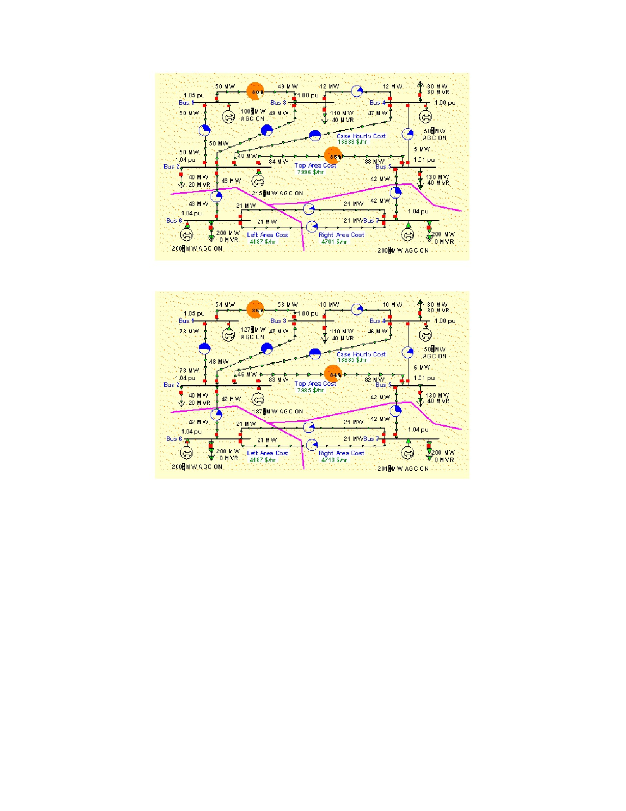
B7OPF Case Solved using LP OPF
B7OPF Case Solved using LP OPF with 100 Cost Segments for Generators
700

PowerWorld Simulator Add-on Tools
OPF Example - Marginal Costs
Using the OPF solution from the previous page, select LP OPF, Bus Records to view the bus marginal costs and LP
OPF, OPF Area Records to view the area marginal costs. The results should be as shown below.
Seven Bus Case Bus and Area Marginal Costs
Note that the marginal costs for all the buses in an area are identical to the area's MW marginal cost. This is the
expected result for systems without any line congestion. The area MW marginal costs are not identical. This is
because currently each area is indepedently enforcing its own MW interchange. In the next example we'll jointly
dispatch the three areas by combining them into a single super area.
701

OPF Example - Super Areas
To jointly dispatch the three areas we'll first combine them into a single super area. To setup the super area first
select LP OPF > OPF Super Area Records to display the OPF Super Area Records display (alternatively you could
also use the Case Information > Super Area display). To enter a new super area right click on the "None Defined"
entry in the first row of the display to show the display's local menu. Select Insert. This displays the super area dialog
. In the Name field enter a name for the new super area, "ThreeAreas." Then select the Add New button to create a
new super area. To add the three areas to the new super area enter "1-3" in the New Area #'s field and then select
Add New Areas by Number (alternatively you could select the areas from the New Area Name list). Also, to enable
the super area for control, set the Super Area Control Options field (AGC Status) to Optimal Power Flow (OPF.)
Before resolving the OPF lets temporarily disable enforcement of line MVA constraints. You can do this from the
Constraint Options page of the OPF Options dialog. Check the Disable Line/Transformer MVA Limit Enforcement.
Also, now would be a good time to save the changes. To avoid overwriting the existing B7OPF file, select File > Save
Case As to save the case (pwb and pwd f iles) with a different name, say B7OPFSA (SA for super area).
Select LP OPF > Primal LP to resolve the OPF. The results should be as shown below.
OPF Solution with Super Area WITHOUT Enforcing Line MVA Constraints
With the super area the individual area interchange constraints are no longer enforced. This permits the free
interchange of power between the areas, resulting in an overall decrease in the total case hourly cost from $ 16,885 /
hr to $ 16,251 / hr. View the OPF Bus Records display to v erify that all the bus marginal costs are identical, equal to $
17.10 / MWh. Of course the key problem with solving the system using the super area is that now there are line
violations. These violations will be removed next by enforcing the line MVA constraints.
702

PowerWorld Simulator Add-on Tools
OPF Example - Enforcing Line MVA Constraints
To remove the line MVA violations go back to the Constraint Options Page of the LP OPF > OPF Options Dialog.
Uncheck the Disable Line/Transformer MVA Limit Enforcement.
Now resolve the LP OPF, enforcing the line constraints. The resultant solution is shown below.
OPF Solution with Super Area WITH Line MVA Constraint Enforcement
With line constraint enforcement active the OPF optimally redispatches the generation taking into account the line
MVA limits. However enforcing these line constraints comes at a cost. Notice that the total case hourly cost has
increased from $ 16,251 / hr to $ 16,553 / hr, which is still substantially less than the $ 16,885 / hr figure we had for the
case without the superarea.
Enforcing the line constraints also has an impact on the bus marginal costs, shown below.
Impact of Line MVA Enforcement on the Bus Marginal Costs
The actual marginal cost of enforcing the line constraint can also be viewed on the LPOPF, OPF Line/Transformer
MVA Records display. The MVA Marg. Cost tells the marginal cost of enforcing the constraint, expressed in units of $
/ MVA / hr. Right-click on the MVA Marg Cost field header to sort the display using this field.
703

704
PowerWorld Simulator Add-on Tools
Storing OPF Data
Load LP OPF Data
Select LP OPF > Load LP OPF Data to load LP OPF specific fields into the case from the specified *.pwo text file.
Note, the LP OPF specific fields are saved with the case in the pwb file. The pwo files should therefore only be used
for transferring the opf specific data between cases or for the user to manually change the data using a text editor.
Existing OPF specified data can be stored in a *.pwo text file using the LP OPF, Store LP OPF Data menu command.
705
Store LP OPF Data
Select LP OPF > Store LP OPF Data to store LP OPF specific fields from the case into the specified *.pwo text file.
Note, the LP OPF specific fields are saved with the case in the pwb file. The pwo files should therefore only be used
for transferring the opf specific data between cases or f or the user to manually change the data using a text editor.
Data can be loaded into a case from the *.pwo text file using the LP OPF > Load LP OPF Data menu command.
Security Constrained Optimal Power Flow (SCOPF)
Security Constrained Optimal Power Flow Overview
Note: The SCOPF option in PowerWorld Simulator is only available if you have purchased the SCOPF and
OPF add-ons to the base package. To learn more about the SCOPF, please feel free to read through the
information contained in these help files. Contact PowerWorld Corporation for details about ordering the
SCOPF and OPF versions of Simulator.
The optimal power flow (OPF) algorithm has the purpose of minimizing an objective function (usually total operation
cost) by changing different system controls while meeting power balance constraints and enforcing base case
operating limits. The secure operation of a power system though requires that there be no unmanageable contingency
violations, either. Thus, the minimization of the objective function requires considering contingencies. This is
achieved using a security constrained optimal power flow (SCOPF) algorithm.
During the SCOPF solution process the algorithm determines the optimal state of the system by iterating between
solving a standard power flow and solving a linear program that changes the system controls to remove contingency
violations.
The SCOPF algorithm makes control adjustments to the base case (pre-contingency condition) to prevent violations in
the post-contingency conditions. If enough controls are available in the system, the solution minimizes the objective
function and the system enforces contingency violations. If the system does not have enough controls, then some
violations may be persistent under certain contingencies. Those represent unenforceable constraints, which result in
high bus marginal costs.
The commands and options for the SCOPF are accessed using the LP OPF > Security Constrained OPF option.
The SCOPF function uses the OPF options defined in the OPF Options dialog and the contingency settings specified
in the contingency analysis dialog. Please read through the OPF and the contingency analysis help for more
information about these settings. We encourage you to become familiar with Simulator OPF and the contingency
analysis tool before running SCOPF simulations. Other commands in the SCOPF dialog are used to specify the base
case solution process and for accessing the SCOPF results.
706
PowerWorld Simulator Add-on Tools
SCOPF Objective Function
The SCOPF objective function uses the function defined in the OPF settings. There are two objective functions in
Simulator: Minimum Cost and Minimum Control Change. Minimum Cost attempts to minimize the sum of the total
generation costs in specified areas or super areas. Minimum Control Change attempts to minimize the change in the
generation in the specified areas or super areas. The objective function is set up in the OPF options dialog.
The result of the SCOPF will be different from the OPF solution because the SCOPF meets additional inequality
constraints associated with the contingency violations.
707
SCOPF Dialog
The SCOPF dialog allows the user to control options of Security Constrained OPF, as well as to access the
optimization results.
The SCOPF can be run from this dialog using the Run Full Se curity Constrained OPF button at the top of the form.
There are three pages of information included in this form:
Options
Results
LP Solution Details.
708
PowerWorld Simulator Add-on Tools
SCOPF Solution Process
The SCOPF involves three major steps that can be solved either automatically or manually from the SCOPF control
dialog:
· Initialization to setup the SCOPF LP tableau and the control structures
· Contingency analysis calculation and storage of control sensitivities associated with each contingency violation
· SCOPF iterations, which include an LP solution and a power flow solution. During each LP step in the LP
routine, the algorithm enforces the newest most severe contingency violation. After each violation is processed,
all of the unprocessed violations are updated. This step is crucial since often resolving the most severe violation
resolves numerous other violations. For instance, a single line might be overloaded in a number of
contingencies: fixing the worst contingency fixes the others as well. On the other hand, processing some
violations may result in new violations. Currently SCOPF does not check for new violations, which would require
a new contingency analysis solution. Care must be taken during the outer loop since the corrected violations will
no longer show up as binding and hence will be excluded from the SCOPF LP tableau. The contingency
violations are listed in the CTG Violations dialog.
The SCOPF terminates when all the contingency violations have been processed. Note that the user can rerun the
SCOPF by repeating the solution process if they want to verify the contingency violation enforcement at the new
optimal operating point.
709
SCOPF Results
The Results page of the Security Constrained Optimal Power Flow form provides information on the results of the
latest SCOPF solution, including the contingency violations included, the marginal price details, and the marginal
control details.
710
PowerWorld Simulator Add-on Tools
SCOPF Equality and Inequality Constraints
Two general types of constraints are involved in the SCOPF solution: equality and inequality constraints. Equality
constraints are constraints that have to be enforced. That is, they are always "binding". For example in the SCOPF,
as well as in the OPF and in the power flow, the real and reactive power balance equations at system buses must
always be satisfied (at least to within a user specified tolerance). In contrast, inequality constraints may or may not be
binding. For example, a line MVA flow under a certain contingency may or may not be at its limit.
The SCOPF problem is solved by iterating between a power flow solution and a contingency constrained LP solution,
some of the constraints are enforced during the power flow solution and some constraints are enforced during the LP
solution. The constraints enforced during the power flow are, for the most part, the constraints that are enforced
during any power flow solution. These include the bus power balance equations, the generator voltage set point
constraints, and the reactive power limits on the generators. What differentiates the SCOPF from a standard power
flow and from the OPF are the constraints that are explicitly enforced by the LP solver. These include the following
constraints:
Equality Constraints
Inequality Constraints
711
SCOPF Equality Constraints
The SCOPF equality constraints are the s ame as the OPF equality constraints: Area MW interchange, bus MW and
Mvar power balance, Generator voltage setpoint and super area MW interchange.
712
PowerWorld Simulator Add-on Tools
SCOPF Inequality Constraints
The following classes of inequality constraints are enforced during the SCOPF solution.
Generator real power limits
Generator real power limits are enforced during the SCOPF LP solution.
Generator reactive power limits
Generator reactive power limits are enforced during the SCOPF LP solution.
Interface MW Limits
Interface MW limits are enforced during the SCOPF solution. Interfaces are used to represent the aggregate flow
through a number of different devices. During the SCOPF the MW post-contingency flow through the interface is
constrained to be less than or equal to a user specified percentage of its limit, provided the interface is active for
enforcement. For an interface to be active for enforcement the following three conditions must be met:
· Interface enforcement must not be disabled for the case. This field can be set from either the OPF
constraintsOPF_Options_Constraint_Options dialog or the OPF interfacesOPF_Interface_Records info display.
As default, the interface enforcement is not disabled. Note that interface flow is limited to a percent of its limit as
specified by the interface's Limit Monitoring SettingsLimit_Monitoring_Settings.
· Interface enforcement must be active for at least one of the interface's areas. Note, an interface is assumed to
be in each area that contains at least one of its components. This field can be set from the OPF Area
RecordsOPF_Area_Records display. Note: the default is that interface enforcement is not active, so be sure to
activate this if you want these cons traints enforced.
· Enforcement must be active for each individual interface. This field can be specified from the OPF Interface
RecordsOPF_Interface_Records display or in the Limit Monitoring SettingsLimit_Monitoring_Settings dialog.
The default is active.
Each interface that is active for enforcement is modeled as an inequality constraint, which may be either binding or
not binding. If the constraint is not binding then it does not impact the solution. If a constraint is binding then it has
an associated marginal cost of contingency enforcement. When manually solving the SCOPF one can skip a
contingency violation associated to the interface by setting the Include field of the SCOPF CTG Violations dialog to
No.
Transmission Line and Transformer (Branch) MVA Limits
Transmission line and transformer (branch) MVA limits are enforced during the SCOPF solution. During the LP the
post-contingency branch line flow is constrained to be less than or equal to a user specified percentage of its limit,
provided the branch is active for enforcement. For a branch to be active for enforcement the following three
conditions must be met:
· Line/Transformer enforcement must not be disabled for the case. This field can be set from either the OPF
constraints dialogOPF_Options_Constraint_Options or the OPF Line/Transformer
RecordsOPF_Line_Transformer_Records display. The default is that case line/transformer enforcement is not
disabled. Also note that the branch flow is limited to a percent of its limit as specified by the branch's Limit
Monitoring SettingsLimit_Monitoring_Settings.
· Branch enforcement must be active for the branch's area. Enforcement For tie-lines must be active for either
area. This field can be set from the OPF Line/Transformer RecordsOPF_Line_Transformer_Records display.
The default is that branch enforcement is not active, so be sure to activate this if you want these constraints
enforced.
· Enforcement must be active for each individual branch. This field can be set from the OPF Line/Transformer
Records display or in the Limit Monitoring Settings Dialog. The default is active.
Each branch that is active for enforcement is modeled as an inequality constraint, which may be either binding or
not binding under contingency conditions. If the constraint is not binding then it does not impact the solution. If a
constraint is binding then it has an associated marginal cost of enforcing the contingency constraint, which is shown
on the SCOPF Bus Marginal Price Details dialog. When manually solving the SCOPF one can skip a contingency
violation associated to the branch by setting the Include field of the SCOPF CTG Violations dialog to No.
713
SCOPF Control
The control dialog allows the user to manually or automatically run a SCOPF simulation and visualize the execution of
the simulation. The SCOPF solution process involves three steps: base case solution and initialization, contingency
analysis, and SCOPF iterations.
Run Full Security Constrained OPF
Press this button to run the three steps of the SCOPF solution automatically. The SCOPF will solve the base case
using the selected method, will use the currently stored list of contingencies during the contingency analysis step,
and will take the CA results and sensitivities to iterate in order to obtain the optimal solution that minimizes cost and
enforces contingency violations.
Options
Maximum Number of Outer Loop Iterations
Indicates the number of maximum outer loop iterations. The outer loop iterations determines how many times the
contingency analysis will be re-run following a successful SCOPF dispatch. In this manner, Simulator will look for
new violations that may occur due to the new generation dispatch. The original violations considered will not be
considered again, only new violations will be examined. The presumption is that the original violations will not
resurface. Resolving the contingency analysis independent of the SCOPF routine after the SCOPF dispatch is
acquired will indicate if any earlier violations resurfaced from the final iterated SCOPF dispatch.
Consider Binding Contingent Violations from Last SCOPF Solution
When checked, this option ensures that the contingent violations from the last SCOPF solution are included in the
current SCOPF solution. This option is helpful in preventing the SCOPF from hunting between having a constraint
binding in one solution, and resolving with it not binding in a later solution because it was previously remedied. This
option should generally always be checked, unless the user is sure that the previous solution has no bearing on the
current solution, such as having made major changes to the system since the previous solution.
Initialize SCOPF with Previously Binding Constraints
When checked, this option results in the SCOPF solution process starts with the exact same LP tableau from the
last solution. This can make for fairly fast solutions (recognizing that the contingency analysis needs to be
resolved) when the changes to the system are small. Simulator automatically uses this option when doing multiple
outer loops of the SCOPF. This option allows the user to solve the outer loops (set the outer loop counter to 1) by
repeatedly solving the SCOPF manually, potentially making modifications between solutions if desired.
Set Solution as Contingency Analysis Reference Case
Check this field to set the solution of the SCOPF as the contingency analysis reference. If the system has enough
controls to remove all the contingency violations, a rerun of the contingency analysis using the SCOPF solution as
the reference should report no branch violations.
Maximum Number of Contingency Violations Allow Per Element
Specify the maximum number of contingency v iolations that the SCOPF analysis should allow per element.
Basecase Solution Method
Specifies whether the solution of the base case is performed using the power flow algorithm or the optimal power
flow algorithm. The selection will affect the initial conditions of the system and consequently the contingency
analysis results and the sensitivities used by the LP solver. Currently the SCOPF does not resolve the contingency
analysis during the optimization since this is computationally expensive. See the SCOPF solution process for
details.
Handling of Contingent Violations Due to Radial Load
It is often common when computing a security constrained OPF to have violations occur on branches due to radial
load. In these instances, there is no way to adjust c ontrols to continue to serve the load, without overloading the
serving element. Therefore you can choose how contingent violations of this type should be handled by the
SCOPF. You can choose to flag them but not include them in the SCOPF, ignore them completely, or include the
violations in the SCOPF. Note that if you include the violations in the SCOPF, the SCOPF algorithm will not be able
to remove the violation on the element via generation dispatch. However, it may be able to do so if the load in
question has a load benefit curve defined and is available for load shed dispatch in the SCOPF routine.
DC SCOPF Options
The DC options given for the SCOPF revolve around the treatment of Line Outage Distribution Factors (LODF)
during the DC SCOPF solution. You can choose to discard the LODFs when the SCOPF is finished, store them in
memory (lost when Simulator is closed,) or in memory and in the PWB file (if saved.)
If the LODFs have been stored and you wish to clear them (they can require quite a bit of RA M depending on the
number of contingencies and size of the case,) you can press the button labeled Clear Stored Contingency
Analysis LODFs .
714
PowerWorld Simulator Add-on Tools
Number of Outer Loop Iterations
The number of outer loop iterations required to solve the SCOPF.
Number of Contingent Violations
Number of violations from the contingency analysis portion of the solution, which are used to attempt to determine
the security constrained dispatch.
SCOPF Start Time, SCOPF End Time
Physical time when the SCOPF solution process started and finished.
Total Solution Time (Seconds)
Length of time needed to determine the SCOPF solution.
Total LP Iterations
Total number of Linear Programming iterations necessary to determine the SCOPF solution.
Number of Active Contingencies
Is the number of contingencies included in the SCOPF simulation Specific contingencies may be excluded from the
simulation in the contingency analysis dialog by changing the skip field of a contingency to YES. The contingency
analysis dialog can be conveniently accessed from the SCOPF control dialog.
View Contingency Analysis Form
Clicking this button shows the contingency analysis dialog.
Contingency Analysis Results
This window allows the user to monitor the details of the contingency analysis step. During contingencies, the
outage actions, the solution of each contingency, and the solution of the CA run are reported.
715
SCOPF CTG Violations
The contingency violations page is available from the Results tab of the Security Constrained Optimal Power Flow
form. The display lists the results from the latest contingency analysis run including the violations that were included
in the SCOPF and the final error for each violation. This dialog may change if the user reruns the SCOPF by solving
the contingency analysis using the SCOPF solution as contingency analysis reference. Right click any where in the
display to copy a portion or all of the display to the Window's clipboard, or to print the results.
The display shows the following fields:
Contingency Name
This is the contingency label. By default single line contingencies start with an "L", single generator outages with a
"G", and single transformer outages start with an "X".
Category
Currently, the SCOPF considers only branch and interface violations. Thus, the category of the contingencies
should be branch MVA or Interface.
Element
Shows information about the specific element that presented the violation. When the violation occurs in a branch,
this column includes the identifiers of the sending and receiving ends of the branch, the circuit, and the direction of
the violating flow. Since Interfaces are directed, this field will present only the interface name in the case of
violating interfaces.
Value
The percentage flow that appears in the branch during the contingency prior to optimization. If this number is larger
than the scaled limit, the violation needs to be removed.
Scaled Limit
The scaled limit corresponds to the Line/Transformer Percentage specified in the limit monitoring settings dialog.
By specifying this limit to be higher than 100% some of the contingency violations might be effectively relaxed.
Sometimes this helps the OPF and the SCOPF obtain a feasible solution. On the other hand, it is often required to
analyze the performance of the system if branches would have higher ratings.
New Value
The percentage flow that appears in the branch during the contingency after SCOPF optimization. If this number is
larger than the scaled limit, the contingency violation has not been removed and it is therefore unenforceable. If the
value is equal to the scaled limit, then the contingency violation constraint would be binding. If the value is smaller
than the scaled limit, the contingency violation has been removed.
Error
The difference between the new value and the scaled limit. If the error is positive, the line is unenforceable. If the
error is zero, the constraint is binding. Negative errors indicate that the violations have been corrected.
Included
Indicates if the contingency violation was included as a constraint in the SCOPF solution.
Marginal Cost
Indicates the cost associated with the contingency violation. If the constraint is unenforceable, the marginal cost is
assigned arbitrarily as a high value in the OPF constraint options dialog.
Unenforceable
Indicates whether the contingency violations is unenforceable, i.e., the system has not enough controls to relieve
the branch overload when the contingency occurs.
Skip Violation?
Change this field to NO if the contingency violations should not be included as a SCOPF constraint. This is
sometimes useful in order to analyze the effect of the contingency violation in the SCOPF solution. This field may
be toggled when doing a manual SCOPF solution.
716
PowerWorld Simulator Add-on Tools
SCOPF LP Solution Details
The LP Solution Details page of the Security Constrained Optimal Power Flow form provides information on the linear
program solution of the SCOPF, including a list of All LP Variables, LP Basic Variables, and LP Basis Matrix. This
information applies to the linear programming tableau solution method.
717